Code
set.seed(1234)
Fake <- data.frame(matrix(rnorm(n=(100*8)), nrow=100, ncol=8))
Err <- rnorm(n=100, mean=0, sd=8)
Y <- 5 + 2*Fake$X2 - 3*Fake$X8 + Err
Fake <- cbind(Fake, Err, Y)Simulations can also be used to evaluate models. One of the most popular examples is target shuffling. Target shuffling has been around for a long time, but has recently been brought back to popularity by Dr. John Elder from Elder Research. Target shuffling is when you randomly reorder the target variables values among the sample, while keeping the predictor variable values fixed. An example of this is shown below:

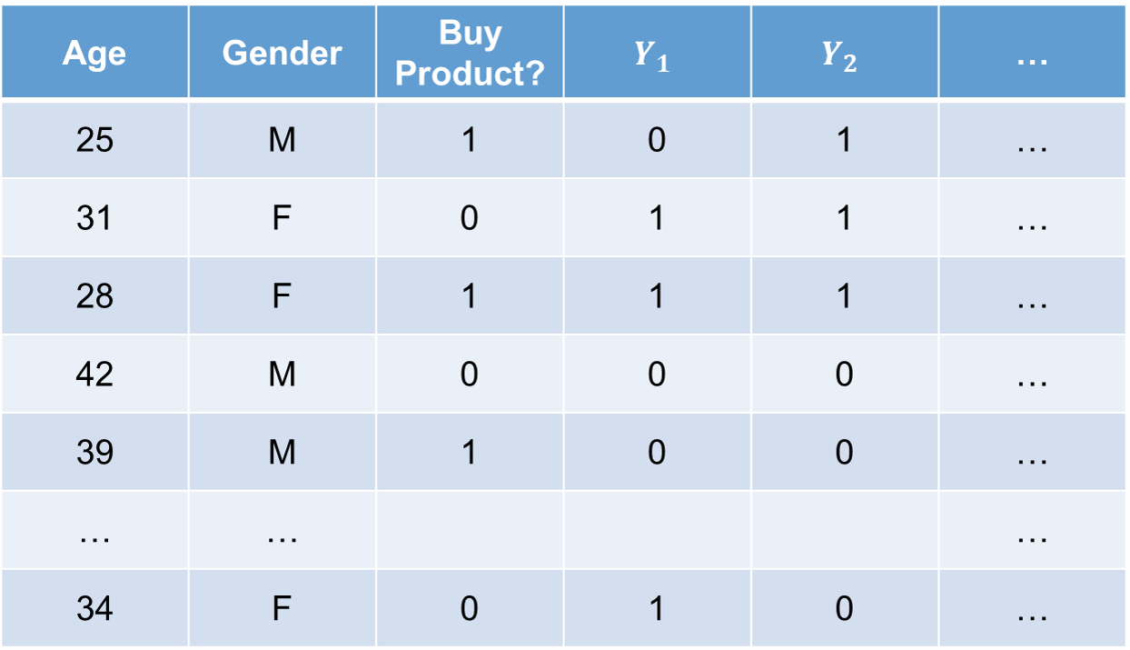
In the above picture, we are using two variables to predict the target variable if you are going to buy a product. Those two variables are age and gender. However, we have also shuffled the values (same number of categories, just different order) of the target variable to create columns \(Y_1\), \(Y_2\), etc.
The goal of target shuffling is to build a model for each of the target variables - both the one real one and all the shuffled ones. We will then record the same model evaluation metric from each shuffle to see how well our model performs compared to the random data. The shuffling should remove the pattern from the data, but some pattern may still exist in some of the shuffles due to randomness. This will help us evaluate how well our model did as compared to random as well as tell us the probability we arrived at our results just by chance.
The following sections outline two examples.
We are going to randomly generate 8 variables that follow a normal distribution with a mean of 0 and standard deviation of 8. However, only two of these variables will be related to our target variable:
\[ Y = 5 + 2X_2 - 3X_8 + \varepsilon \]
We are going to perform a target shuffle on our target variable \(Y\) and look at a couple of things. First, the adjusted \(R^2\) value from our model compared to the target shuffled (random data) models. Second, the number of significant variables in the target shuffled (random data) models. Remember, there should be no relationship when we shuffle our target so our adjusted \(R^2\) should be close to zero in the target shuffled models and there should not really be any significant variables in the target shuffled models.
Let’s see this example in each of our softwares!
Similar to the omitted variable bias example above, we will need to generate predictor variables first and then calculate our target variable from the two that should be in the model. Our first step is to generate a matrix of 100 observations (rows) of 8 variables (columns) all with normal distributions with mean 0 and standard deviation of 1. We will save this as a data frame Fake. Next, we have the Err object that is our model error term, \(\varepsilon\), that has a normal distribution with mean of 0 and standard deviation of 8. Now we create our target variable \(Y\) as defined above and combine all these columns into one data frame Fake.
The next step is to shuffle the target variable. We will create another matrix with 100 observations (rows) and 1000 columns - one column for each shuffle. With a for loop we can randomly sample from a uniform distribution using the runif function. We will then order our Y column by these uniform random numbers. This will essentially randomly order the target variable. We do this repeatedly and store these in each column of our 1000 shuffle columns. We rename these columns (Y.1, Y.2, …) and combine them all into one new data frame.
Now we just run our 1,001 and linear regressions. The for loop will run a linear regression using the lm function on all the shuffled columns. The summary function’s adj.r.squared element is then stored for each target shuffled model. Lastly, we also run the true regression model and get its adjusted \(R^2\) using the same procedure. This makes our 1,001 adjusted \(R^2\) metrics. Let’s visualize these adjusted \(R^2\) values on a histogram.
R.sq.A <- rep(0,sim)
for(i in 1:sim){
R.sq.A[i] <- summary(lm(Fake[,10+i] ~ Fake$X1 + Fake$X2 + Fake$X3 + Fake$X4
+ Fake$X5 + Fake$X6 + Fake$X7 + Fake$X8))$adj.r.squared
}
True.Rsq.A <- summary(lm(Fake$Y ~ Fake$X1 + Fake$X2 + Fake$X3 + Fake$X4
+ Fake$X5 + Fake$X6 + Fake$X7 + Fake$X8))$adj.r.squared
hist(c(R.sq.A,True.Rsq.A), breaks=50, col = "blue", main='Distribution of Adjusted R-Squared Values', xlab='Adjusted R-Squared')
abline(v = True.Rsq.A, col="red", lwd=2)
mtext("True Model", at=True.Rsq.A, col="red")
Our model out performs all of the other models. However, despite not expecting any good results from the shuffled data, we see some adjusted \(R^2\) values that almost reach 0.2. Again, this is due to random chance. This allows us to test our model to see if we just got a data set that is lucky, or if we really have some interesting findings.
Let’s see how many variables were significant in each of our shuffled models. Remember, the data has been completely shuffled so there shouldn’t be any significant variables. To do this, use a similar for loop as above, but instead of looking at the adj.r.squared element of the summary function, we look at the \(4^{th}\) column of our coefficient element - the p-values for our variables. We then count the number of times the p-value was below a significance level of 0.05.
(Intercept) Fake$X1 Fake$X2 Fake$X3 Fake$X4 Fake$X5
1000 51 46 53 53 43
Fake$X6 Fake$X7 Fake$X8
53 46 50
0 1 2 3 4
675 264 53 7 1 
Most of the time we see that no variables were significant, but out of the 1000 shuffles, each variable was significant about 50 times. This isn’t surprising as the goal of a significance level of 0.05 in a hypothesis test is to make an error 5% of the time. However, sometimes these errors happened together. Seven out of the 1,000 shuffled models had three significant variables in the model. One even had four significant variables. This is all due to random chance.
Similar to the omitted variable bias example above, we will need to generate predictor variables first and then calculate our target variable from the two that should be in the model. Our first step is to generate a matrix of 100 observations (rows) of 8 variables (columns) all with normal distributions with mean 0 and standard deviation of 1. We will save this as a data frame Fake. Next, we have the Err object that is our model error term, \(\varepsilon\), that has a normal distribution with mean of 0 and standard deviation of 8. Now we create our target variable \(Y\) as defined above and combine all these columns into one data frame Fake.
import numpy as np
import pandas as pd
np.random.seed(12345)
Fake = np.random.normal(loc = 0, scale = 1, size = 8*100).reshape(100, 8)
Fake = pd.DataFrame(Fake)
Fake.columns = ['X1', 'X2', 'X3', 'X4', 'X5', 'X6', 'X7', 'X8']
Fake['Y'] = 5 + 2*Fake['X2'] - 3*Fake['X8'] + np.random.normal(loc = 0, scale = 6, size = 100)The next step is to shuffle the target variable. We will create another matrix with 100 observations (rows) and 1000 columns - one column for each shuffle. With a for loop we can randomly sample from a uniform distribution using the random.uniform function. We will then order our Y column by these uniform random numbers. This will essentially randomly order the target variable. We do this repeatedly and store these in each column of our 1000 shuffle columns. We rename these columns (Y1, Y2, …) and combine them all into one new data frame.
Now we just run our 1,001 and linear regressions. The for loop will run a linear regression using the OLS function (from stasmodels.api) on all the shuffled columns. The rsquared_adj element is then stored for each target shuffled model. Lastly, we also run the true regression model and get its adjusted \(R^2\) using the same procedure. This makes our 1,001 adjusted \(R^2\) metrics. Let’s visualize these adjusted \(R^2\) values on a histogram.
import statsmodels.api as sm
X = Fake.iloc[:, range(8)]
X = sm.add_constant(X)
R_sq_A = []
for i in range(1000):
Y = Fake.iloc[:, i + 9]
model = sm.OLS(Y, X).fit()
rsa = model.rsquared_adj
R_sq_A.append(rsa)
Y = Fake.iloc[:, 8]
model = sm.OLS(Y, X).fit()
rsa = model.rsquared_adj
R_sq_A.append(rsa)
R_sq_A = pd.DataFrame(R_sq_A)
R_sq_A.columns = ['R_sq_A']
import seaborn as sns
ax = sns.histplot(data = R_sq_A)
ax.set_title('Distribution of Adjusted R-Squared Values')
ax.set_xlabel("Adjusted R-Squared")
ax.axvline(x = rsa, color = "red")
Our model out performs all of the other models. However, despite not expecting any good results from the shuffled data, we see some adjusted \(R^2\) values that almost reach 0.2. Again, this is due to random chance. This allows us to test our model to see if we just got a data set that is lucky, or if we really have some interesting findings.
Let’s see how many variables were significant in each of our shuffled models. Remember, the data has been completely shuffled so there shouldn’t be any significant variables. To do this, use a similar for loop as above, but instead of looking at the rsquared_adj element, we look at the pvalues element - the p-values for our variables. We then count the number of times the p-value was below a significance level of 0.05.
const 1000
X1 47
X2 41
X3 48
X4 39
X5 51
X6 66
X7 52
X8 41
dtype: int640
0 683
1 256
2 55
3 5
4 1
Name: count, dtype: int64Most of the time we see that no variables were significant, but out of the 1000 shuffles, each variable was significant about 50 times. This isn’t surprising as the goal of a significance level of 0.05 in a hypothesis test is to make an error 5% of the time. However, sometimes these errors happened together. Five out of the 1,000 shuffled models had three significant variables in the model. One even had four significant variables. This is all due to random chance.
Similar to the omitted variable bias example above, we will need to generate predictor variables first and then calculate our target variable from the two that should be in the model. Our first step is to generate a dataset of 100 observations (rows) of 8 variables (columns) all with normal distributions with mean 0 and standard deviation of 1. Next, we have the Err object that is our model error term, \(\varepsilon\), that has a normal distribution with mean of 0 and standard deviation of 8. Now we create our target variable \(Y\) as defined above and combine all these columns into one dataset Fake using the DATA step and the RAND function with the Normal option. Don’t forget the OUTPUT statement to store your DO loop results at each iteration.
data Fake;
do obs = 1 to 100;
call streaminit(12345);
X1 = RAND('Normal', 0, 1);
X2 = RAND('Normal', 0, 1);
X3 = RAND('Normal', 0, 1);
X4 = RAND('Normal', 0, 1);
X5 = RAND('Normal', 0, 1);
X6 = RAND('Normal', 0, 1);
X7 = RAND('Normal', 0, 1);
X8 = RAND('Normal', 0, 1);
Err = RAND('Normal', 0, 8);
Y = 5 + 2*X2 - 3*X8 + Err;
output;
end;
run;The next step is to shuffle the target variable. We will do this using a MACRO we create called shuffle. This MACRO will use a DATA step to create a random sample from a uniform distribution using the RAND function with the Uniform option. We will then order our Y column by these uniform random numbers using PROC SORT. This will essentially randomly order the target variable. We use another DATA step to merge this new randomly shuffled dataset with our original one using the MERGE statement. We then use PROC DATASETS to delete this random shuffle dataset to not clog up our memory. Next we create another MACRO called sim_shuffle that runs the shuffleMACRO a specified number of times. We will run ours 500 times.
%macro shuffle(sim);
data shuffle_∼
set Fake;
Uni = RAND('Uniform');
Y_&sim = Y;
keep Y_&sim Uni;
run;
proc sort data=shuffle_∼
by Uni;
run;
data Fake;
merge Fake shuffle_∼
drop Uni;
run;
proc datasets noprint;
delete shuffle_∼
run;
quit;
%mend shuffle;
%macro sim_shuffle(sim);
%do i = 1 %to ∼
%shuffle(&i);
%end;
%mend sim_shuffle;
%sim_shuffle(500);Now we just run our 1001 and linear regressions. The PROC REG procedure will run a linear regression on the original target \(Y\) and on all the shuffled columns. We will use the SELECTION = BACKWARD option to backward select our significant variables with a significance level of 0.05. We store the adjusted \(R^2\) values using the OUTEST option. Let’s visualize these adjusted \(R^2\) values on a histogram with PROC SGPLOT.
proc reg data=Fake noprint outest=Rsq_A;
model Y Y_1-Y_500 = X1-X8 / selection=backward slstay=0.05 adjrsq;
run;
quit;
proc sgplot data=Rsq_A;
title 'Distribution of Adjusted R-Squared';
histogram _ADJRSQ_;
refline 0.178 / axis=x label='True Model' lineattrs=(color=red thickness=2);
keylegend / location=inside position=topright;
run;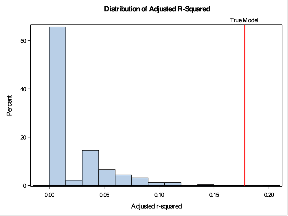
Our model out performs all of the other models. However, despite not expecting any good results from the shuffled data, we see some adjusted \(R^2\) values that almost reach 0.2. Again, this is due to random chance. This allows us to test our model to see if we just got a data set that is lucky, or if we really have some interesting findings.
Let’s see how many variables were significant in each of our shuffled models. Remember, the data has been completely shuffled so there shouldn’t be any significant variables. To do this, use a similar for loop as above, but instead of looking at the adj.r.squared element of the summary function, we look at the \(4^{th}\) column of our coefficient element - the p-values for our variables. We then count the number of times the p-value was below a significance level of 0.05.
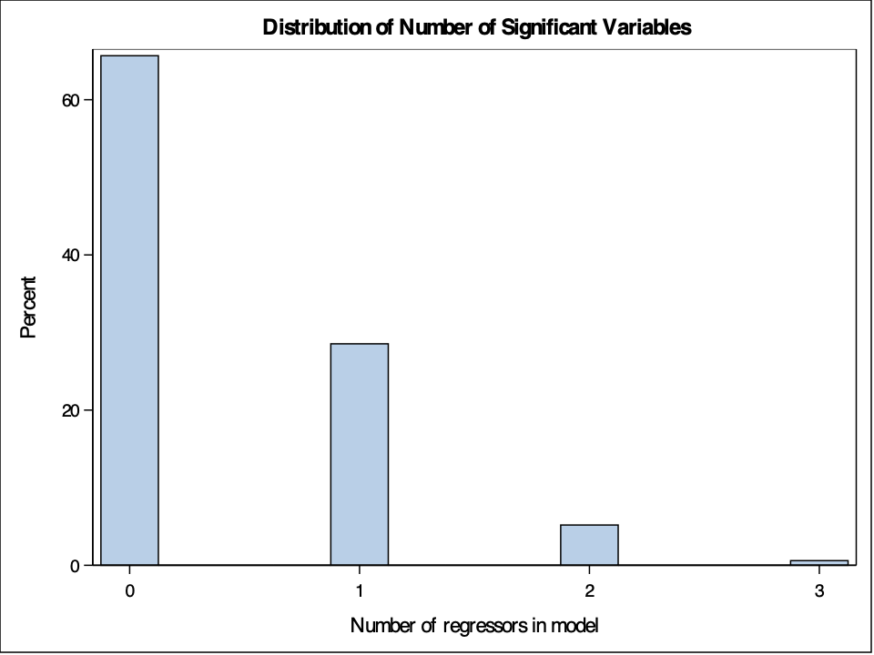
Most of the time we see that no variables were significant, but out of the 1000 shuffles, each variable was significant about 50 times. This isn’t surprising as the goal of a significance level of 0.05 in a hypothesis test is to make an error 5% of the time. However, sometimes these errors happened together. Seven out of the 1000 shuffled models had three significant variables in the model. This is all due to random chance.
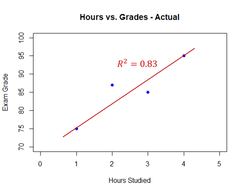
Target shuffling is essentially a simulation version of permutation analysis. This can be easily seen with an example using student grades. Imagine there were 4 students in a class. One studied 1 hour for an exam, another 2 hours, another 3 hours, and the last one 4 hours. Their grades on the exam were 75, 87, 85, and 95 respectively. If you were to plot these grades on a scatter plot and run a linear regression you would have the following:

This model has an \(R^2 = 0.83\). What if the professor randomly shuffled these grades among the four students? How many different ways can four students get the grades of 75, 87, 85, and 95? There are 24 possible ways which are all listed below:

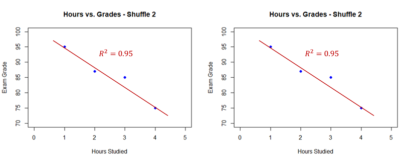
Of these 24 grades, there are 3 possible combinations that produce a linear regression with an \(R^2\) value that is greater than or equal to our actual data. Two of these are plotted below (the third is the inverse of our above plot):

Therefore, there are 4 combinations of grades that produce a regression with an \(R^2\) that is greater than or equal to our actual data - a chance of \(4/24 = 1/6 = 16.67\%\). This problem didn’t need to be target shuffled as it was easy to calculate all possible combinations of the target variable, \(4! = 24\). However, what if we had 40 students instead of 4? The number of permutations of the target variable increases tremendously (\(40! = 8.16 \times 10^{47}\)). This is the value of target shuffling. Target shuffling is essentially a simulated sampling of permutation analysis.
---
title: "Model Evaluation - Target Shuffling"
format:
html:
code-fold: show
code-tools: true
editor: visual
---
```{r}
#| include: false
library(reticulate)
use_condaenv("r-main")
```
# Target Shuffling
Simulations can also be used to evaluate models. One of the most popular examples is **target shuffling**. Target shuffling has been around for a long time, but has recently been brought back to popularity by Dr. John Elder from [Elder Research](https://www.elderresearch.com/). Target shuffling is when you randomly reorder the target variables values among the sample, while keeping the predictor variable values fixed. An example of this is shown below:
{fig-align="center" width="7in"}
In the above picture, we are using two variables to predict the target variable if you are going to buy a product. Those two variables are age and gender. However, we have also shuffled the values (same number of categories, just different order) of the target variable to create columns $Y_1$, $Y_2$, etc.
The goal of target shuffling is to build a model for each of the target variables - both the one real one and all the shuffled ones. We will then record the same model evaluation metric from each shuffle to see how well our model performs compared to the random data. The shuffling should remove the pattern from the data, but some pattern may still exist in some of the shuffles due to randomness. This will help us evaluate how well our model did as compared to random as well as tell us the probability we arrived at our results just by chance.
The following sections outline two examples.
# Fake Data
We are going to randomly generate 8 variables that follow a normal distribution with a mean of 0 and standard deviation of 8. However, only two of these variables will be related to our target variable:
$$
Y = 5 + 2X_2 - 3X_8 + \varepsilon
$$
We are going to perform a target shuffle on our target variable $Y$ and look at a couple of things. First, the adjusted $R^2$ value from our model compared to the target shuffled (random data) models. Second, the number of significant variables in the target shuffled (random data) models. Remember, there should be no relationship when we shuffle our target so our adjusted $R^2$ should be close to zero in the target shuffled models and there should not really be any significant variables in the target shuffled models.
Let's see this example in each of our softwares!
::: {.panel-tabset .nav-pills}
## R
Similar to the omitted variable bias example above, we will need to generate predictor variables first and then calculate our target variable from the two that should be in the model. Our first step is to generate a matrix of 100 observations (rows) of 8 variables (columns) all with normal distributions with mean 0 and standard deviation of 1. We will save this as a data frame *Fake*. Next, we have the *Err* object that is our model error term, $\varepsilon$, that has a normal distribution with mean of 0 and standard deviation of 8. Now we create our target variable $Y$ as defined above and combine all these columns into one data frame *Fake*.
```{r}
set.seed(1234)
Fake <- data.frame(matrix(rnorm(n=(100*8)), nrow=100, ncol=8))
Err <- rnorm(n=100, mean=0, sd=8)
Y <- 5 + 2*Fake$X2 - 3*Fake$X8 + Err
Fake <- cbind(Fake, Err, Y)
```
The next step is to shuffle the target variable. We will create another matrix with 100 observations (rows) and 1000 columns - one column for each shuffle. With a `for` loop we can randomly sample from a uniform distribution using the `runif` function. We will then order our Y column by these uniform random numbers. This will essentially randomly order the target variable. We do this repeatedly and store these in each column of our 1000 shuffle columns. We rename these columns (*Y.1*, *Y.2*, ...) and combine them all into one new data frame.
```{r}
sim <- 1000

Y.Shuffle <- matrix(0, nrow=100, ncol=sim)
for(j in 1:sim){
  Uniform <- runif(100)
  Y.Shuffle[,j] <- Y[order(Uniform)]
}

Y.Shuffle <- data.frame(Y.Shuffle)
colnames(Y.Shuffle) <- paste('Y.',seq(1:sim),sep="")

Fake <- data.frame(Fake, Y.Shuffle)
```
Now we just run our 1,001 and linear regressions. The `for` loop will run a linear regression using the `lm` function on all the shuffled columns. The `summary` function's `adj.r.squared` element is then stored for each target shuffled model. Lastly, we also run the true regression model and get its adjusted $R^2$ using the same procedure. This makes our 1,001 adjusted $R^2$ metrics. Let's visualize these adjusted $R^2$ values on a histogram.
```{r}
R.sq.A <- rep(0,sim)
for(i in 1:sim){
  R.sq.A[i] <- summary(lm(Fake[,10+i] ~ Fake$X1 + Fake$X2 + Fake$X3 + Fake$X4
                          + Fake$X5 + Fake$X6 + Fake$X7 + Fake$X8))$adj.r.squared
}
True.Rsq.A <- summary(lm(Fake$Y ~ Fake$X1 + Fake$X2 + Fake$X3 + Fake$X4
                         + Fake$X5 + Fake$X6 + Fake$X7 + Fake$X8))$adj.r.squared

hist(c(R.sq.A,True.Rsq.A), breaks=50, col = "blue", main='Distribution of Adjusted R-Squared Values', xlab='Adjusted R-Squared')
abline(v = True.Rsq.A, col="red", lwd=2)
mtext("True Model", at=True.Rsq.A, col="red")
```
Our model out performs all of the other models. However, despite not expecting any good results from the shuffled data, we see some adjusted $R^2$ values that almost reach 0.2. Again, this is due to random chance. This allows us to test our model to see if we just got a data set that is lucky, or if we really have some interesting findings.
Let's see how many variables were significant in each of our shuffled models. Remember, the data has been completely shuffled so there shouldn't be any significant variables. To do this, use a similar `for` loop as above, but instead of looking at the `adj.r.squared` element of the `summary` function, we look at the $4^{th}$ column of our `coefficient` element - the p-values for our variables. We then count the number of times the p-value was below a significance level of 0.05.
```{r}
P.Values <- NULL
for(i in 1:sim){
  P.V <- summary(lm(Fake[,10+i] ~ Fake$X1 + Fake$X2 + Fake$X3 + Fake$X4
                    +                           + Fake$X5 + Fake$X6 + Fake$X7 + Fake$X8))$coefficients[,4]
  P.Values <- rbind(P.Values, P.V)
}

Sig <- P.Values < 0.05

colSums(Sig)
table(rowSums(Sig)-1)
hist(rowSums(Sig)-1, breaks=25, col = "blue", main='Count of Significant Variables Per Model', xlab='Number of Sig. Variables')
```
Most of the time we see that no variables were significant, but out of the 1000 shuffles, each variable was significant about 50 times. This isn't surprising as the goal of a significance level of 0.05 in a hypothesis test is to make an error 5% of the time. However, sometimes these errors happened together. Seven out of the 1,000 shuffled models had three significant variables in the model. One even had four significant variables. This is all due to random chance.
## Python
Similar to the omitted variable bias example above, we will need to generate predictor variables first and then calculate our target variable from the two that should be in the model. Our first step is to generate a matrix of 100 observations (rows) of 8 variables (columns) all with normal distributions with mean 0 and standard deviation of 1. We will save this as a data frame *Fake*. Next, we have the *Err* object that is our model error term, $\varepsilon$, that has a normal distribution with mean of 0 and standard deviation of 8. Now we create our target variable $Y$ as defined above and combine all these columns into one data frame *Fake*.
```{python}
import numpy as np
import pandas as pd

np.random.seed(12345)

Fake = np.random.normal(loc = 0, scale = 1, size = 8*100).reshape(100, 8)
Fake = pd.DataFrame(Fake)
Fake.columns = ['X1', 'X2', 'X3', 'X4', 'X5', 'X6', 'X7', 'X8']

Fake['Y'] = 5 + 2*Fake['X2'] - 3*Fake['X8'] + np.random.normal(loc = 0, scale = 6, size = 100)
```
The next step is to shuffle the target variable. We will create another matrix with 100 observations (rows) and 1000 columns - one column for each shuffle. With a `for` loop we can randomly sample from a uniform distribution using the `random.uniform` function. We will then order our Y column by these uniform random numbers. This will essentially randomly order the target variable. We do this repeatedly and store these in each column of our 1000 shuffle columns. We rename these columns (*Y1*, *Y2*, ...) and combine them all into one new data frame.
```{python}
#| warning: false
#| message: false
sim = 1000

iteration = 1
for i in range(sim):
  data = Fake['Y']
  data = pd.DataFrame(data)
  data['uni'] = np.random.uniform(size = 100)
  data = data.sort_values(by = ['uni'])
  data = data.reset_index()

  col_name = 'Y' + str(iteration)
  Fake.loc[:, col_name] = data['Y']
  iteration = iteration + 1
```
Now we just run our 1,001 and linear regressions. The `for` loop will run a linear regression using the `OLS` function (from `stasmodels.api`) on all the shuffled columns. The `rsquared_adj` element is then stored for each target shuffled model. Lastly, we also run the true regression model and get its adjusted $R^2$ using the same procedure. This makes our 1,001 adjusted $R^2$ metrics. Let's visualize these adjusted $R^2$ values on a histogram.
```{python}
#| warning: false
#| message: false
import statsmodels.api as sm

X = Fake.iloc[:, range(8)]
X = sm.add_constant(X)

R_sq_A = []
for i in range(1000):
  Y = Fake.iloc[:, i + 9]
  model = sm.OLS(Y, X).fit()
  rsa = model.rsquared_adj
  R_sq_A.append(rsa)

Y = Fake.iloc[:, 8]
model = sm.OLS(Y, X).fit()
rsa = model.rsquared_adj
R_sq_A.append(rsa)

R_sq_A = pd.DataFrame(R_sq_A)
R_sq_A.columns = ['R_sq_A']

import seaborn as sns

ax = sns.histplot(data = R_sq_A)
ax.set_title('Distribution of Adjusted R-Squared Values')
ax.set_xlabel("Adjusted R-Squared")
ax.axvline(x = rsa, color = "red")
```
Our model out performs all of the other models. However, despite not expecting any good results from the shuffled data, we see some adjusted $R^2$ values that almost reach 0.2. Again, this is due to random chance. This allows us to test our model to see if we just got a data set that is lucky, or if we really have some interesting findings.
Let's see how many variables were significant in each of our shuffled models. Remember, the data has been completely shuffled so there shouldn't be any significant variables. To do this, use a similar `for` loop as above, but instead of looking at the `rsquared_adj` element, we look at the `pvalues` element - the p-values for our variables. We then count the number of times the p-value was below a significance level of 0.05.
```{python}
Y = Fake.iloc[:, 9]
model = sm.OLS(Y, X).fit()
Pval = pd.DataFrame(model.pvalues)

for i in range(999):
  Y = Fake.iloc[:, i + 10]
  model = sm.OLS(Y, X).fit()
  Pval2 = model.pvalues
  Pval = pd.concat([Pval, Pval2], axis = 1)

Pval = Pval < 0.05

Pval.sum(axis = 1)
Sig = Pval.sum(axis = 0) - 1

Sig = pd.DataFrame(Sig)
Sig.value_counts()
```
Most of the time we see that no variables were significant, but out of the 1000 shuffles, each variable was significant about 50 times. This isn't surprising as the goal of a significance level of 0.05 in a hypothesis test is to make an error 5% of the time. However, sometimes these errors happened together. Five out of the 1,000 shuffled models had three significant variables in the model. One even had four significant variables. This is all due to random chance.
## SAS
Similar to the omitted variable bias example above, we will need to generate predictor variables first and then calculate our target variable from the two that should be in the model. Our first step is to generate a dataset of 100 observations (rows) of 8 variables (columns) all with normal distributions with mean 0 and standard deviation of 1. Next, we have the *Err* object that is our model error term, $\varepsilon$, that has a normal distribution with mean of 0 and standard deviation of 8. Now we create our target variable $Y$ as defined above and combine all these columns into one dataset *Fake* using the `DATA` step and the `RAND` function with the `Normal` option. Don't forget the `OUTPUT` statement to store your `DO` loop results at each iteration.
```{r}
#| eval: false
data Fake;
    do obs = 1 to 100;
        call streaminit(12345);
        X1 = RAND('Normal', 0, 1);
        X2 = RAND('Normal', 0, 1);
        X3 = RAND('Normal', 0, 1);
        X4 = RAND('Normal', 0, 1);
        X5 = RAND('Normal', 0, 1);
        X6 = RAND('Normal', 0, 1);
        X7 = RAND('Normal', 0, 1);
        X8 = RAND('Normal', 0, 1);
        Err = RAND('Normal', 0, 8);

        Y = 5 + 2*X2 - 3*X8 + Err;

        output;
    end;
run;
```
The next step is to shuffle the target variable. We will do this using a MACRO we create called *shuffle*. This MACRO will use a `DATA` step to create a random sample from a uniform distribution using the `RAND` function with the `Uniform` option. We will then order our Y column by these uniform random numbers using `PROC SORT`. This will essentially randomly order the target variable. We use another `DATA` step to merge this new randomly shuffled dataset with our original one using the `MERGE` statement. We then use `PROC DATASETS` to delete this random shuffle dataset to not clog up our memory. Next we create another MACRO called *sim_shuffle* that runs the *shuffle*MACRO a specified number of times. We will run ours 500 times.
```{r}
#| eval: false
%macro shuffle(sim);
    data shuffle_∼
        set Fake;
        Uni = RAND('Uniform');
        Y_&sim = Y;
        keep Y_&sim Uni;
    run;

    proc sort data=shuffle_∼
        by Uni;
    run;

    data Fake;
        merge Fake shuffle_∼
        drop Uni;
    run;

    proc datasets noprint;
        delete shuffle_∼
    run;
    quit;
%mend shuffle;

%macro sim_shuffle(sim);
    %do i = 1 %to ∼
        %shuffle(&i);
    %end;
%mend sim_shuffle;

%sim_shuffle(500);
```
Now we just run our 1001 and linear regressions. The `PROC REG` procedure will run a linear regression on the original target $Y$ and on all the shuffled columns. We will use the `SELECTION = BACKWARD` option to backward select our significant variables with a significance level of 0.05. We store the adjusted $R^2$ values using the `OUTEST` option. Let's visualize these adjusted $R^2$ values on a histogram with `PROC SGPLOT`.
```{r}
#| eval: false
proc reg data=Fake noprint outest=Rsq_A;
    model Y Y_1-Y_500 = X1-X8 / selection=backward slstay=0.05 adjrsq;
run;
quit;

proc sgplot data=Rsq_A;
    title 'Distribution of Adjusted R-Squared';
    histogram _ADJRSQ_;
    refline 0.178 / axis=x label='True Model' lineattrs=(color=red thickness=2);
    keylegend / location=inside position=topright;
run;
```
{fig-align="center" width="7in"}
Our model out performs all of the other models. However, despite not expecting any good results from the shuffled data, we see some adjusted $R^2$ values that almost reach 0.2. Again, this is due to random chance. This allows us to test our model to see if we just got a data set that is lucky, or if we really have some interesting findings.
Let's see how many variables were significant in each of our shuffled models. Remember, the data has been completely shuffled so there shouldn't be any significant variables. To do this, use a similar `for` loop as above, but instead of looking at the `adj.r.squared` element of the `summary` function, we look at the $4^{th}$ column of our `coefficient` element - the p-values for our variables. We then count the number of times the p-value was below a significance level of 0.05.
```{r}
#| eval: false
proc sgplot data=Rsq_A;
    title 'Distribution of Number of Significant Variables';
    histogram _IN_;
run;
```
{fig-align="center" width="7in"}
Most of the time we see that no variables were significant, but out of the 1000 shuffles, each variable was significant about 50 times. This isn't surprising as the goal of a significance level of 0.05 in a hypothesis test is to make an error 5% of the time. However, sometimes these errors happened together. Seven out of the 1000 shuffled models had three significant variables in the model. This is all due to random chance.
:::
# Student Grade Analogy
Target shuffling is essentially a simulation version of permutation analysis. This can be easily seen with an example using student grades. Imagine there were 4 students in a class. One studied 1 hour for an exam, another 2 hours, another 3 hours, and the last one 4 hours. Their grades on the exam were 75, 87, 85, and 95 respectively. If you were to plot these grades on a scatter plot and run a linear regression you would have the following:
{fig-align="center" width="7in"}
This model has an $R^2 = 0.83$. What if the professor randomly shuffled these grades among the four students? How many different ways can four students get the grades of 75, 87, 85, and 95? There are 24 possible ways which are all listed below:
{fig-align="center" width="8in"}
Of these 24 grades, there are 3 possible combinations that produce a linear regression with an $R^2$ value that is greater than or equal to our actual data. Two of these are plotted below (the third is the inverse of our above plot):
{fig-align="center" width="8in"}
Therefore, there are 4 combinations of grades that produce a regression with an $R^2$ that is greater than or equal to our actual data - a chance of $4/24 = 1/6 = 16.67\%$. This problem didn't need to be target shuffled as it was easy to calculate **all** possible combinations of the target variable, $4! = 24$. However, what if we had 40 students instead of 4? The number of permutations of the target variable increases tremendously ($40! = 8.16 \times 10^{47}$). This is the value of target shuffling. Target shuffling is essentially a simulated sampling of permutation analysis.