| Variable | Description |
|---|---|
| Age_oldest_tr | Age of oldest trade |
| App_id | Application ID |
| Bad | Godd/Bad loan |
| Bankruptcy | Bankruptcy (1) or not (0) |
| Bureau_score | Bureau score |
| Down_pyt | Amount of down payment on vehicle |
| Loan_amt | Amount of loan |
| Loan_term | How many months vehicle was financed |
| Ltv | Loan to value |
| MSRP | Manufacturer suggested retail price |
| Purch_price | Purchase price of vehicle |
| Purpose | Lease or own |
| Rev_util | Revolving utilization (balance/credit limit) |
| Tot_derog | Total number of derogatory trades (go past due) |
| Tot_income | Applicant’s income |
| Tot_open_tr | Number of open trades |
| Tot_rev_debt | Total revolving debt |
| Tot_rev_line | Total revolving line |
| Tot_rev_tr | Total revolving trades |
| Tot_tr | Total number of trades |
| Used_ind | Used car indicator |
| Weight | Weight variable |
Data Preparation
Defining the Target
When dealing with credit scoring data, the first major hurdle is to define the target variable of default. This might be harder than initially expected. When does someone actually default? Do you wait for the loan to be charged-off by the bank? There were probably plenty of signs before then that the customer would stop paying on their loan.
People use to always use 90 days past due (DPD) as the typical definition of default. If a customer goes 90 days past their due date for a payment on a loan, they would be considered a default. Now, default ranges between 90 and 180 days past due based on the types of loans, business sector, and country regulations. For example, in the United States, 180 days past due is the default standard on mortgage loans.
Discrete vs. Continuous Time
Credit scoring tries to understand the probability of default on a customer (or business). However, default depends on time for its definition. When a customer or business will default is just as valuable as if they will. How we incorporate time into the evaluation of credit scoring is important for this reason.
Accounting for time is typically broken down into two approaches:
Discrete time
Continuous time
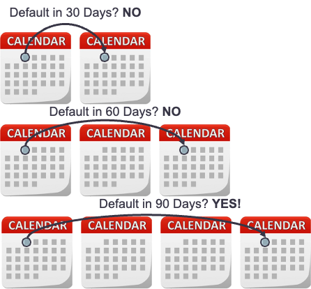
Discrete time evaluates binary decisions on predetermined intervals of time. For example, are you going to default in the next 30, 60, or 90 days. Each of these intervals have a separate binary credit scoring model. This approach is very popular in credit scoring consumers as people don’t actually care about the exact day of default as compared to the number of missed payments. Defaulting at 72 days isn’t needed as long as I know if a consumer defaulted between 60 and 90 days as shown in the picture below with the different models - 30 day, 60 day, 90 day.

These models used together can piece together windows of time where it is believed a consumer will default.
Continuous time evaluates the probability of default as it changes over continuous points in time. Instead of a series of binary classification models, survival analysis models are used for this approach as they can predict the exact day of default as shown in the picture below.

This is more important in credit scoring businesses to determine the exact time a business may declare bankruptcy and default on a loan. This approach is starting to gain more popularity in consumer credit modeling to better help with the amount of capital to keep on hand with consumers defaulting at specific times as compared to windows of time.
Feature Engineering
Predictor Variables
Selecting predictor variables in credit scoring models also takes care. Credit scoring models desire variables that have a high amount of predictability for default, but that isn’t the only criteria. Since regulators will be checking these models, they have to have variables that are easily interpretable from a business stand-point. They also must be reliably and easily collected both now and in the future since you don’t want to make a mistake in a loan decision. These variables also must be though of ethically to ensure that the bank is being fair and equitable to all of their customers.
Feature engineering is an important part of the process for developing good predictor variables. In fact, good feature engineering can replace the need for more advanced modeling techniques that lack the interpretation needed for a good credit scorecard model. Features may be created based on business reasoning, such as the loan to value ratio, the expense to income ratio, or the credit line utilization across time. Variable clustering may also be used to omit variables that are highly dependent on each other.
Sampling
When it comes to sample size, there are no hard, fast rules on how much data is needed for building credit scoring models. The FDIC suggests that samples “normally include at least 1,000 good, 1,000 bad, and 750 rejected applicants.” However, sample size really depends on the overall size of the portfolio, the number of predictor variables being planned for the model, and the number of defaults in the data.
Sampling must also be characteristic of the population to which the scorecard will be applied. For example, if the scorecard is to be applied in the sub-prime lending program, then we must use a sample that captures the characteristics of the sub-prime population targeted. Here are the two main steps for sampling for credit scoring models:
Gather data for accounts opened during a specific time frame.
Monitor the performance of these accounts for another specific length of time to determine if they were good or bad.
This approach raises natural concerns. Accounts that are opened more recently are more similar to account that will be opened in the near future so we don’t want to go too far back in time to sample. However, we want to minimize the chances of missclassifying the performance of the account so we need to monitor the accounts long enough to let them fail. Banks develop cohort graphs to help them determine how long a typical customer takes to default on a loan. Essentially, watch customer accounts and their default rates. When these default rates tend to level off, then a majority of the customers who will have defaulted will be done. This relies on the empirical data that shows that customers that default typically do so early in the life of a loan. From these cohort charts comes the concepts of sample and performance windows.
For example, let’s imagine the typical amount of time a customer takes to default on a loan is 14 months. If our analysis is to be performed on March of this year, we will select our sample from 12-16 months back. This will give us an average of 14 months for our performance window. An example of this is shown below.

Now that our data is set, we can move into truly preparing our variables for modeling.
Data Description
The first thing that we need to do is load up all of the needed libraries in R that we will be using in these course notes.
We will be using the auto loan data to build a credit scorecard for applicants for an auto loan. This credit scorecard predicts the likelihood of default for these applicants. There are actually two data sets we will use. The first is a data set on 5,837 people who were ultimately given auto loans. The variables in the accepts data set are the following:
The accepts data set has actually been oversampled for us because the event of defaulting on the auto loans is only 5% in the population. Our sample has closer to a 20% default rate.