Reject Inference

Background and Legalities

The initial scorecard we built in the last section using only known defaulters and non-defaulters is called a behavioral scorecard since it models the behavior of our current clients. However, the current customers who we accept for a loan are not the same as the “through-the-door” population that applies for a loan. To better comply with regulatory requirements of fairness (from the FDIC, Basel Accords, etc.) we want to develop a scorecard that can generalize better to the entire credit population that applies for a loan.

Reject inference is the process of inferring the status (target variable) of the rejected applicants based on the accepted applicant model in an attempt to use their information to build a scorecard that is representative of the entire population. Reject inference is about solving sampling bias so that the development sample is similar to the population to which the scorecard will be applied.

However, this does not imply that we cannot develop a scorecard model without reject applicants. It is still legally permissible to use these behavioral scorecards to score applicants, however, it is strongly advised to use reject inference whenever possible to protect from biasing the results. This is best summarized by one of my favorite quotes on reject inference:

Raymond Anderson, Head of Scoring at Standard Bank Africa

“My suggestion is to develop the scorecard using what data you have, but start saving rejected applications ASAP.”

Reject Inference Techniques

There are many different techniques to perform reject inference and infer the target variable of default / non-default onto our rejected applicants. Three of the most popular techniques will be discussed in explicit detail below:

Simple / Hard Cut-off Augmentation
Parceling Augmentation
Fuzzy Augmentation

Each of these techniques starts off the same way. First, we take the model that we have built on the accepted applicants and score the rejected applicants to get either the predicted probabilities or the predicted scorecard scores. For the examples below, we will use the predicted probabilities, but the same process applies if you used the predicted scores.

The main difference between each of the techniques is how we use the newly scored rejected applicant dataset.

Simple / Hard Cut-off Augmentation

For the simple / hard cut-off augmentation approach, we take the newly scored observations in your rejected applicant dataset and select a cut-off. A good selection for this cut-off is one that would maximize predictive capability like the Youden Index / Optimal K-S statistic. Although detail is not provided here in this code deck, more information on these techniques can be found in model evaluation section of the Logistic Regression code deck.

Once we select a cut-off, we create a binary variable from this cut-off. On one side of the cut-off we have the predicted defaulters and the other side is the predicted non-defaulters as shown below.

With this newly created binary variable, we have an inferred target variable for our rejected dataset.

Parceling Augmentation

For the parceling augmentation approach, we take the newly scored observations in your rejected applicant dataset and split these observations into bins based those scores / predictions. The idea behind these bins is that you are grouping together observations that have similar attributes. The attributes of these observations are assumed to be about the same because they have similar predictions. Within each of these bins we examine the actual default rate based on the same bin ranges in our accepted dataset. From that default rate we randomly assign each observation to a default or non-default as show below.

Let’s work through a couple of examples. Let’s say that the bin with the highest predicted probability of default has an actual default rate of 25%. We would randomly assign 25% of the observations to default and the rest to non-default.

Another example would be on the opposite end of the spectrum. Imagine the default rate is 1% from the accept dataset of the predictions in the range of the lowest bin from the reject dataset. That means we would randomly assign 1% of the observations in that bin to default and the rest non-default.

Instead of looking at examples with predicted probabilities, we can look at a numerical example with predicted scores instead.

In the example above we can look at a predicted score range from the accepted applicant model of 655 - 665. In that range in the accepted applicant dataset we have 45.5% of our observations as defaulters. That means that we will randomly assign our 190 rejected applicants in that predicted range a value of default 45.5% of the time. This means that approximately 86 of them will be randomly assigned as defaulters, while the rest (104) are assigned as non-defaulters. If you have ranges where there are no accepted applicants, we would assume that all of those observations in the rejected observations are defaulters.

The main idea behind parceling augmentation is that we don’t truly know who would have defaulted and who would not have defaulted. However, instead of completely randomly assigning default or non-default to everyone at the population level, we will randomly assign at a more specific level based on the predictions from our behavioral scorecard model.

With this newly created binary variable, we have an inferred target variable for our rejected dataset.

Fuzzy Augmentation

For the fuzzy augmentation approach, we take the newly scored observations in your rejected applicant dataset and make two separate observations. These two separate observations have one marked as a defaulter and one marked as a non-defaulter. You can think about this as the good and bad representation of each applicant. The predicted probability form the behavioral scorecard model comes into play with the weighting of each observation.

For example, if you have a predicted probability of default of 0.78, then the default observation will have its old weight multiplied by 0.78 and the non-default observation will have its old weight multiplied by 0.22 ($= 1 - 0.78$). The old weight for these observations refers to the weights used in the behavioral scorecard model since we had to oversample to account for the extreme unbalance in our original target variable. If no oversampling was needed, then these old weights would be 1 for every observation before multiplying in the predicted probabilities.

Essentially, with fuzzy augmentation we have a duplicated dataset for our rejected applicants where each rejected applicant is given two observations in this new dataset - both a defaulter and non-defaulter. We just weight these observations differently. For example, if we had 1,000 rejected applicants before, we now have a dataset with 1,000 defaulters and 1,000 non-defaulters for 2,000 total observations.

With this newly created binary variable, we have an inferred target variable for our rejected dataset.

Reject Inference Example

For our example dataset we will use a simple / hard cut-off augmentation example.

Let’s see how to do this with each of our softwares!

Python
R

To create a scored rejected applicant dataset in Python is very easy. We use the same predict_proba function on the Scorecard object that contains the model we developed in the previous section. We can use the rejected applicants dataset as the input to this function to get the predicted probabilities. From there we just set the cut-off. We will use the cut-off of 0.06 determined from the previous section on scorecard model evaluation as the optimal K-S statistic cut-off. Any prediction above 0.06 we will infer a default, while the rest are non-default, using our binary bad variable. The next line calculates the new weight for the observations in our data set accounting for the rare event sampling.

Once we have this inferred target variable for the rejected applicant dataset, we can combine the accepted applicant dataset as well as the rejected applicant dataset. However, we cannot just combine them together without considering how the population looks. The dataset this population was pulled from rejected 30% of all applications. Therefore, our final, combined dataset should keep this same 70% accepted and 30% rejected balance or we will have to reweight our dataset to account for this. To make this balance we are just grabbing the first 1,876 observations from our rejected applicant dataset.

Code

X_r = rejects

rejects["y_pred"] = scorecard.predict_proba(X_r)[:, 1]

rejects["bad"] = (rejects["y_pred"] > 0.06).astype(int)
rejects["weight"] = rejects["bad"].apply(lambda x: 4.75 if x == 0 else 1)

rejects = rejects.drop("y_pred", axis=1)

comb_hard = pd.concat([accepts, rejects.head(1876)], ignore_index=True)

Now we have a combined dataset with a target variable for building our final scorecard model.

Before scoring our rejected applicants, we need to perform the same data transformations on the rejected applicants dataset as we did on the accepted applicant dataset. The following R code generates the same bins for our rejected applicant dataset variables that we had in the accepted applicant dataset so we can score these new observations. It also calculates each applicants scorecard score.

Code

rejects_scored <- rejects
rejects_scored$ltv[is.na(rejects_scored$ltv)] <- median(rejects_scored$ltv, na.rm = TRUE)

rejects_scored <- smbinning.gen(df = rejects_scored, ivout = smb_bureau_score, chrname = "bureau_score_bin")
rejects_scored <- smbinning.gen(df = rejects_scored, ivout = smb_tot_rev_line, chrname = "tot_rev_line_bin")
rejects_scored <- smbinning.gen(df = rejects_scored, ivout = smb_rev_util, chrname = "rev_util_bin")
rejects_scored <- smbinning.gen(df = rejects_scored, ivout = smb_age_oldest_tr, chrname = "age_oldest_tr_bin")
rejects_scored <- smbinning.gen(df = rejects_scored, ivout = smb_tot_derog, chrname = "tot_derog_bin")
rejects_scored <- smbinning.gen(df = rejects_scored, ivout = smb_ltv, chrname = "ltv_bin")
rejects_scored <- smbinning.gen(df = rejects_scored, ivout = smb_tot_tr, chrname = "tot_tr_bin")

Next, we just use the predict function to score the rejected applicant dataset. The first input is the model object from our behavioral model. The newdata = option defines the rejected applicant dataset that we need to score. The type = option defines that we want the predicted probability of default for each observation in the reject dataset. The next two lines of code create a bad and good variable in the rejected applicant dataset based on the optimal cut-off defined in the previous section. The next line calculates the new weight for the observations in our data set accounting for the rare event sampling. Lastly, we combine our newly inferred rejected observations with our original accepted applicants for rebuilding our credit scoring model.

Code

rejects_scored$pred <- predict(initial_score,  newdata = rejects_scored, type = 'response') 

rejects$bad <- as.numeric(rejects_scored$pred > 0.0618)
rejects$weight <- ifelse(rejects$bad == 0, 4.75, 1)

rejects$good <- abs(rejects$bad - 1)

rejects_sample <- rejects[1:1876,]

comb_hard <- rbind(accepts, rejects_sample)

Once you have a target variable, you add the rejected applicant dataset back into the accepted applicant dataset to perform an overall analysis since you now have a target variable for all of the observations - a mix of real and inferred. We will still take the same process as before where we split into training and testing. We still must be careful of the about the weights as we want to keep the accepted to rejected balance the same as the population as we don’t want to overweight the rejected applicants in our final model.

Other Reject Inference Techniques

There are other reject inference techniques that are not as highly recommended:

Assign all rejects to defaulters
Assign rejected applicants randomly to defaulter and non-defaulter based on the whole population default rate
Assign default based on a similar in-house model on different data
Approve all applicants for a certain period of time

Each of the above techniques has their inherent problems. Assigning all rejected applicants to defaulters should only be done when very few people are ever rejected and you are very confident in your process for rejecting a loan application. The downside to completely random assignment at a population level is that it can throw off the model results and is only useful if your current decision process has no consistency. Using other products and their models to predict rejected applicants might be a viable solution. However, just because someone might have a high chance of paying back a car loan doesn’t mean they will also pay back a mortgage at the same rate. This process is also tough to pass through regulators. Lastly, the idea of approving all applicants for a certain period of time might sound good in a controlled experiment kind of world, but there are inherent legality and risk problems with this approach as the customer base will most certainly not be the usual customer base in terms of risk as word gets out that you are approving all loans.

Final Scorecard

The mechanics of building the final scorecard are identical with the initial scorecard creation except that analysis is performed after reject inference. We will still take the same process as before where we split into training and testing, re-bin all of the variables, and rebuild the logistic regression model. The rehashing of the code is not shown here, just the results.

We scored the test dataset and looked at the ROC curve for the final model. This ROC curve happens to be even better than the initial behavioral scorecard. We also have less inherent bias in this model because it was developed using reject inference. This also makes this scorecard model appropriate to use for applications - an application scorecard.

Another popular plot to look at when evaluating test datasets is called a decile plot. This plot bins the predicted scores from the test dataset into 10 equal pieces. In each of these bins we look at the default rate. We would hope that our model had higher default in the lower scores and lower default in the higher scores, which is exactly what we see in the plot below. Careful to make sure that you are correctly counting the defaulters and non-defaulters in your dataset, especially if oversampling was done. As you can see in the code below, we are multiplying the non-defaulters (the 0’s in the bad variable) by 4.75 to match the weights.

Code

test_final["score"] = scorecard.score(test_final)
test_final['decile'] = pd.qcut(test_final["score"], 10, labels = False)

PD = test_final[test_final['bad'] == 1].groupby('decile').size() / (test_final[test_final['bad'] == 0].groupby('decile').size() * 4.75 + test_final[test_final['bad'] == 1].groupby('decile').size())


plt.figure(figsize = (8, 6))
PD.plot(kind = 'bar', color = 'skyblue', edgecolor = 'black')
plt.axhline(y = 0.05, color = 'black', linestyle = '--', linewidth = 2)
plt.text(x = 9, y = 0.06, s = '5% Default', color = 'black', ha = 'right', va = 'bottom', fontsize = 12)

plt.title('Proportion of Default across Deciles of Score')
plt.xlabel('Decile')
plt.ylabel('Proportion of Default')
plt.xticks(rotation = 0)

(array([0, 1, 2, 3, 4, 5, 6, 7, 8, 9]), [Text(0, 0, '0'), Text(1, 0, '1'), Text(2, 0, '2'), Text(3, 0, '3'), Text(4, 0, '4'), Text(5, 0, '5'), Text(6, 0, '6'), Text(7, 0, '7'), Text(8, 0, '8'), Text(9, 0, '9')])

Code

plt.grid(True)
plt.show()

Another common plot to look at is what is called the trade-off plot. The first trade-off plot we are looking at compares the acceptance rate with the default rate at different score cut-offs. The x-axis represents the score cut-off. Any applicant with a score higher than that value on the x-axis is assumed to be a non-defaulter. For every point on the x-axis there is a corresponding acceptance rate and default rate. These allow us to compare decisions. For example, a score cut-off of 550 (approve a loan above 550 and deny below) would result in a default rate of 3.15% and approval rate of 78.2%. That means that our model produces results with a higher acceptance rate than currently at the bank (70%), but with a lower default rate than the current default rate (5%). We can play around with different cut-off values to compare risk at the bank.

Another trade-off plot compares the approval rate against the profit. The same process applies to this plot as the previous plot. We can see that a cut-off of 606 (approve a loan above 606 and deny below) would maximize profit at nearly $9 million. However, we would only be approving 34.6% of applicants. Even though this approval rate would lead to an extra low 1.23% default, we might not be making our applicants happy if we give out so few a number of loans.

Instead of selecting one cut-off, another possible scenario would be to select two cut-offs. For example, anyone with a score below 517 is denied. That score corresponds to our current default rate of 5%. Anyone with a score above 606 is approved since that maximizes profit. Anyone in between those two scores could be passed along to have a person look closer at the application to see if we are willing to take the risk.

Model Extensions

There are downsides of the approaches listed in this code deck. One of the biggest downsides is that we don’t have any interactions in the model created above. However, tree-based algorithms are completely based on interactions. One solution to this problem is a multi-stage model with the following process:

Use a decision tree to predict default.
Look at the first couple of splits.
Build a logistic regression based scorecard in each of these splits / subsets of the data.
The interpretation of the scorecards would not be within each of the splits.

When it comes to other more complicated machine learning models, model interpretation is still key in the world of credit scoring. Applying a scorecard layer on top of these models may help drive interpretations, but regulators are still hesitant. This is especially true when you have different interpretations for different people, which regulators really dislike.

One area for complicated machine learning models would be internal comparison and variable selection. For example, can we build a model that statistically beats our WoE based logistic regression model? If we can, are there certain variables we should be including that the machine learning models say are important but our current model isn’t using. Empirical examples have shown WoE based logistic regression models perform very well in comparison to more complicated approaches.

--- title: "Reject Inference" format: html: code-fold: show code-tools: true editor: visual --- ```{python} #| include: false #| message: false #| error: false #| warning: false import pandas as pd accepts = pd.read_csv("~/Dropbox/IAA/Courses/IAA/Financial Analytics/Code Files/FA-new/data/accepts.csv") rejects = pd.read_csv("~/Dropbox/IAA/Courses/IAA/Financial Analytics/Code Files/FA-new/data/rejects.csv") from sklearn.model_selection import train_test_split train, test = train_test_split(accepts, test_size = 0.25, random_state = 1234) ``` ```{r} #| include: false #| message: false #| error: false #| warning: false library(reticulate) train <- py$train test <- py$test accepts <- py$accepts rejects <- py$rejects accepts$good <- abs(accepts$bad - 1) train$good <- abs(train$bad - 1) train$bankruptcy <- as.factor(train$bankruptcy) train$used_ind <- as.factor(train$used_ind) train$purpose <- as.factor(train$purpose) ``` # Background and Legalities The initial scorecard we built in the last section using only **known** defaulters and non-defaulters is called a **behavioral scorecard** since it models the behavior of our current clients. However, the current customers who we accept for a loan are not the same as the "through-the-door" population that applies for a loan. To better comply with regulatory requirements of fairness (from the FDIC, Basel Accords, etc.) we want to develop a scorecard that can generalize better to the entire credit population that applies for a loan. **Reject inference** is the process of inferring the status (target variable) of the rejected applicants based on the accepted applicant model in an attempt to use their information to build a scorecard that is representative of the entire population. Reject inference is about solving sampling bias so that the development sample is similar to the population to which the scorecard will be applied. However, this does not imply that we cannot develop a scorecard model without reject applicants. It is still legally permissible to use these behavioral scorecards to score applicants, however, it is strongly advised to use reject inference whenever possible to protect from biasing the results. This is best summarized by one of my favorite quotes on reject inference: ::: callout-tip ## Raymond Anderson, Head of Scoring at Standard Bank Africa *"My suggestion is to develop the scorecard using what data you have, but start saving rejected applications ASAP."* ::: # Reject Inference Techniques There are many different techniques to perform reject inference and infer the target variable of default / non-default onto our rejected applicants. Three of the most popular techniques will be discussed in explicit detail below: 1. Simple / Hard Cut-off Augmentation 2. Parceling Augmentation 3. Fuzzy Augmentation Each of these techniques starts off the same way. First, we take the model that we have built on the accepted applicants and score the rejected applicants to get either the predicted probabilities or the predicted scorecard scores. For the examples below, we will use the predicted probabilities, but the same process applies if you used the predicted scores.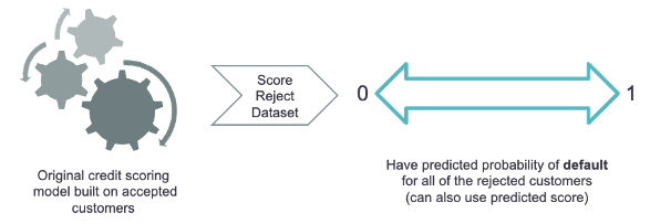 ![](image/RejectInf_Beg.png){fig-align="center" width="6.11in"} The main difference between each of the techniques is how we use the newly scored rejected applicant dataset. ## Simple / Hard Cut-off Augmentation For the simple / hard cut-off augmentation approach, we take the newly scored observations in your rejected applicant dataset and select a cut-off. A good selection for this cut-off is one that would maximize predictive capability like the Youden Index / Optimal K-S statistic. Although detail is not provided here in this code deck, more information on these techniques can be found in model evaluation section of the [Logistic Regression](https://www.ariclabarr.com/logistic-regression/part_5_assess.html#classification-metrics) code deck. Once we select a cut-off, we create a binary variable from this cut-off. On one side of the cut-off we have the predicted defaulters and the other side is the predicted non-defaulters as shown below.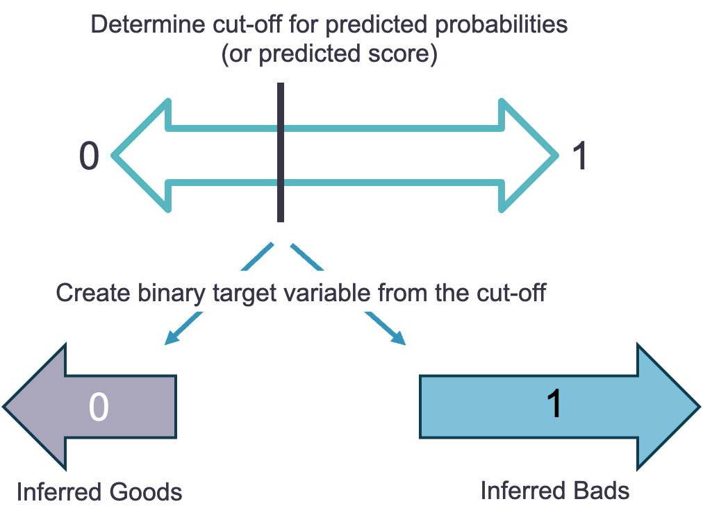 ![](image/RejectInf_Hard.png){fig-align="center" width="5.39in"} With this newly created binary variable, we have an inferred target variable for our rejected dataset. ## Parceling Augmentation For the parceling augmentation approach, we take the newly scored observations in your rejected applicant dataset and split these observations into bins based those scores / predictions. The idea behind these bins is that you are grouping together observations that have similar attributes. The attributes of these observations are assumed to be about the same because they have similar predictions. Within each of these bins we examine the actual default rate based on the same bin ranges in our accepted dataset. From that default rate we randomly assign each observation to a default or non-default as show below.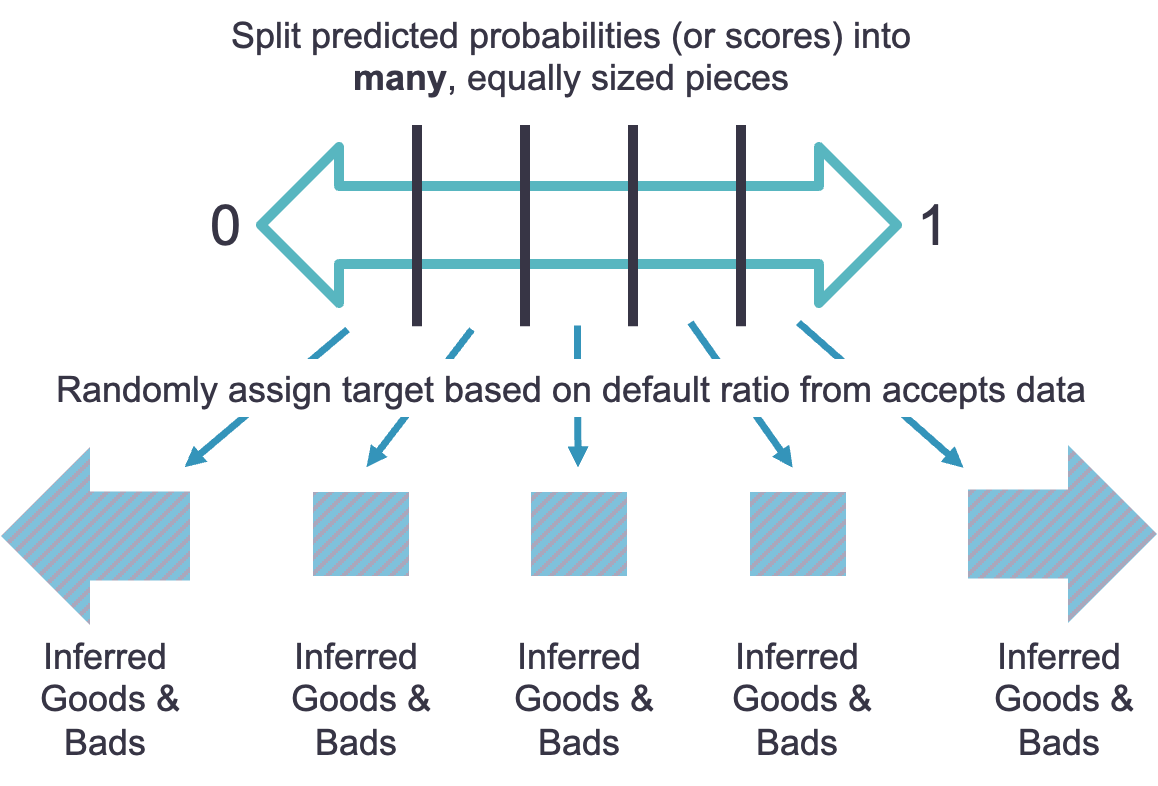 ![](image/RejectInf_Par.png){fig-align="center" width="5.9in"} Let's work through a couple of examples. Let's say that the bin with the highest predicted probability of default has an actual default rate of 25%. We would randomly assign 25% of the observations to default and the rest to non-default.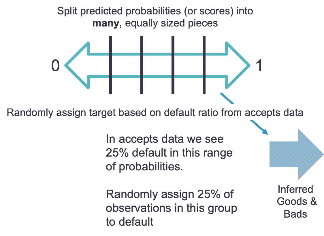 ![](image/RejectInf_Par2.png){fig-align="center" width="5.49in"} Another example would be on the opposite end of the spectrum. Imagine the default rate is 1% from the accept dataset of the predictions in the range of the lowest bin from the reject dataset. That means we would randomly assign 1% of the observations in that bin to default and the rest non-default.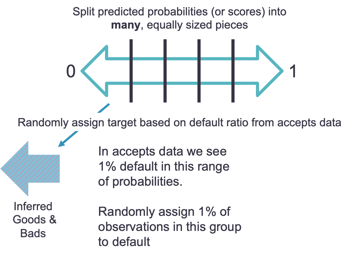 ![](image/RejectInf_Par3.png){width="5.42in"}Instead of looking at examples with predicted probabilities, we can look at a numerical example with predicted scores instead.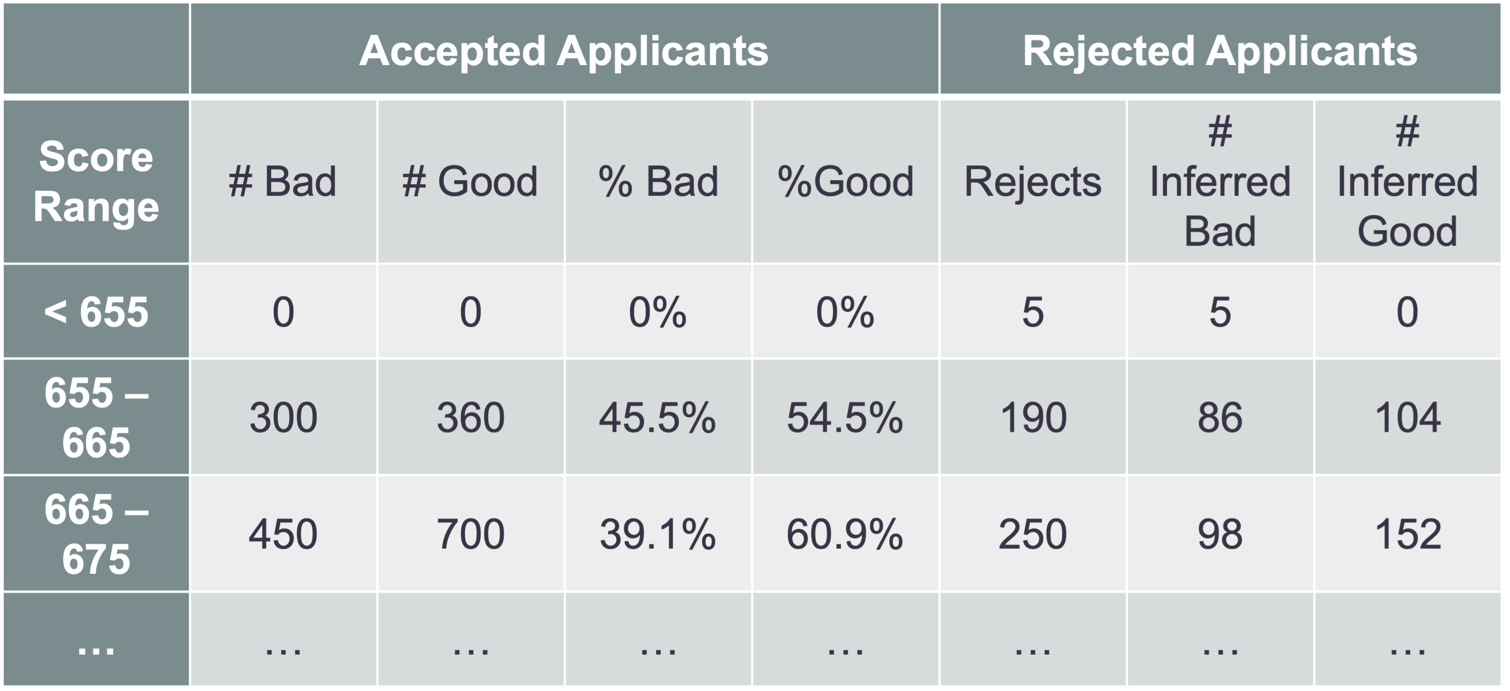 ![](image/RejectInf_Par4.png){fig-align="center" width="8.76in"} In the example above we can look at a predicted score range from the accepted applicant model of 655 - 665. In that range in the accepted applicant dataset we have 45.5% of our observations as defaulters. That means that we will randomly assign our 190 rejected applicants in that predicted range a value of default 45.5% of the time. This means that approximately 86 of them will be randomly assigned as defaulters, while the rest (104) are assigned as non-defaulters. If you have ranges where there are no accepted applicants, we would assume that all of those observations in the rejected observations are defaulters. The main idea behind parceling augmentation is that we don't truly know who would have defaulted and who would not have defaulted. However, instead of completely randomly assigning default or non-default to everyone at the population level, we will randomly assign at a more specific level based on the predictions from our behavioral scorecard model. With this newly created binary variable, we have an inferred target variable for our rejected dataset. ## Fuzzy Augmentation For the fuzzy augmentation approach, we take the newly scored observations in your rejected applicant dataset and make two separate observations. These two separate observations have one marked as a defaulter and one marked as a non-defaulter. You can think about this as the good and bad representation of each applicant. The predicted probability form the behavioral scorecard model comes into play with the weighting of each observation.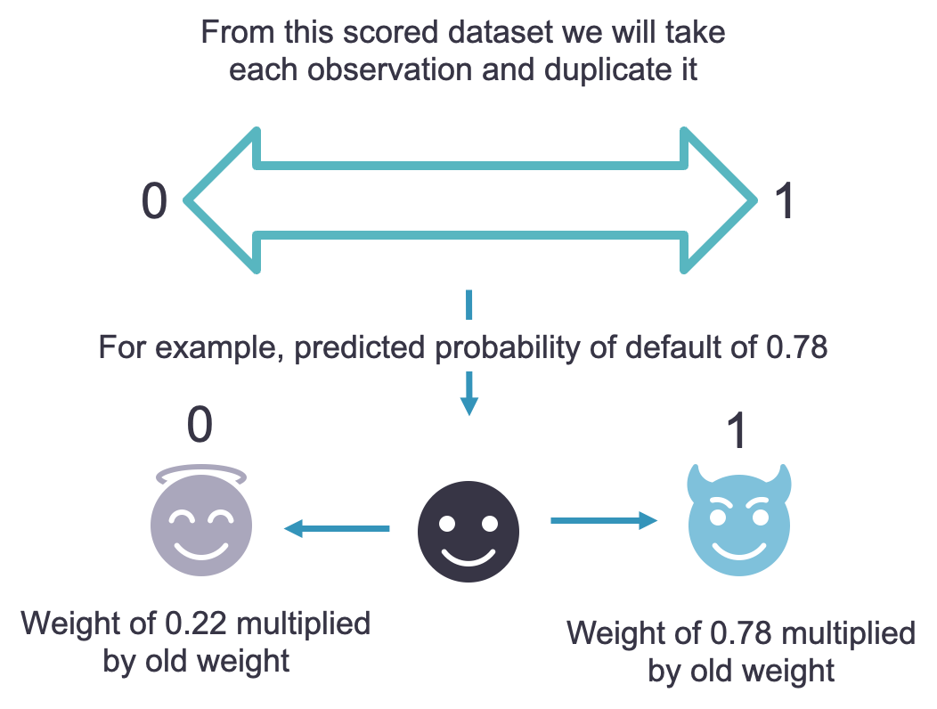 ![](image/RejectInf_Fuz.png){fig-align="center" width="5.28in"} For example, if you have a predicted probability of default of 0.78, then the default observation will have its old weight multiplied by 0.78 and the non-default observation will have its old weight multiplied by 0.22 ($= 1 - 0.78$). The old weight for these observations refers to the weights used in the behavioral scorecard model since we had to oversample to account for the extreme unbalance in our original target variable. If no oversampling was needed, then these old weights would be 1 for every observation before multiplying in the predicted probabilities. Essentially, with fuzzy augmentation we have a duplicated dataset for our rejected applicants where each rejected applicant is given two observations in this new dataset - both a defaulter and non-defaulter. We just weight these observations differently. For example, if we had 1,000 rejected applicants before, we now have a dataset with 1,000 defaulters and 1,000 non-defaulters for 2,000 total observations.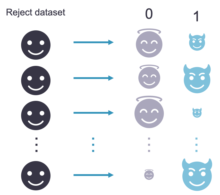 ![](image/RejectInf_Fuz2.png){fig-align="center" width="4.51in"} With this newly created binary variable, we have an inferred target variable for our rejected dataset. ## Reject Inference Example For our example dataset we will use a simple / hard cut-off augmentation example. Let's see how to do this with each of our softwares! ::: {.panel-tabset .nav-pills} ## Python To create a scored rejected applicant dataset in Python is very easy. We use the same `predict_proba` function on the `Scorecard` object that contains the model we developed in the previous section. We can use the rejected applicants dataset as the input to this function to get the predicted probabilities. From there we just set the cut-off. We will use the cut-off of 0.06 determined from the previous section on scorecard model evaluation as the optimal K-S statistic cut-off. Any prediction above 0.06 we will infer a default, while the rest are non-default, using our binary *bad* variable. The next line calculates the new weight for the observations in our data set accounting for the rare event sampling. Once we have this inferred target variable for the rejected applicant dataset, we can combine the accepted applicant dataset as well as the rejected applicant dataset. However, we cannot just combine them together without considering how the population looks. The dataset this population was pulled from rejected 30% of all applications. Therefore, our final, combined dataset should keep this same 70% accepted and 30% rejected balance or we will have to reweight our dataset to account for this. To make this balance we are just grabbing the first 1,876 observations from our rejected applicant dataset. ```{python} #| include: false #| message: false #| warning: false #| error: false import numpy as np import pandas as pd from sklearn.linear_model import LogisticRegression from optbinning import BinningProcess from optbinning import Scorecard colnames = list(train.columns[0:20]) X = train[colnames] y = train["bad"] selection_criteria = {"iv": {"min": 0.1, "max": 1}} bin_proc = BinningProcess(colnames, selection_criteria = selection_criteria, categorical_variables = ["bankruptcy", "purpose", "used_ind"]) estimator = LogisticRegression(solver = "lbfgs") scorecard = Scorecard(binning_process = bin_proc, estimator = estimator, scaling_method = "pdo_odds", scaling_method_params = {"pdo": 20, "scorecard_points": 600, "odds": 50}) scorecard.fit(X, y, sample_weight = train["weight"]) ``` ```{python} #| message: false #| warning: false #| error: false X_r = rejects rejects["y_pred"] = scorecard.predict_proba(X_r)[:, 1] rejects["bad"] = (rejects["y_pred"] > 0.06).astype(int) rejects["weight"] = rejects["bad"].apply(lambda x: 4.75 if x == 0 else 1) rejects = rejects.drop("y_pred", axis=1) comb_hard = pd.concat([accepts, rejects.head(1876)], ignore_index=True) ``` Now we have a combined dataset with a target variable for building our final scorecard model. ## R Before scoring our rejected applicants, we need to perform the same data transformations on the rejected applicants dataset as we did on the accepted applicant dataset. The following R code generates the same bins for our rejected applicant dataset variables that we had in the accepted applicant dataset so we can score these new observations. It also calculates each applicants scorecard score. ```{r} #| include: false #| message: false #| warning: false #| error: false library(smbinning) smb_bureau_score <- smbinning(df = train, y = "good", x = "bureau_score") smb_tot_rev_line <- smbinning(df = train, y = "good", x = "tot_rev_line") smb_rev_util <- smbinning(df = train, y = "good", x = "rev_util") smb_age_oldest_tr <- smbinning(df = train, y = "good", x = "age_oldest_tr") smb_tot_derog <- smbinning(df = train, y = "good", x = "tot_derog") smb_ltv <- smbinning(df = train, y = "good", x = "ltv") smb_tot_tr <- smbinning(df = train, y = "good", x = "tot_tr") train <- smbinning.gen(df = train, ivout = smb_bureau_score, chrname = "bureau_score_bin") train <- smbinning.gen(df = train, ivout = smb_tot_rev_line, chrname = "tot_rev_line_bin") train <- smbinning.gen(df = train, ivout = smb_rev_util, chrname = "rev_util_bin") train <- smbinning.gen(df = train, ivout = smb_age_oldest_tr, chrname = "age_oldest_tr_bin") train <- smbinning.gen(df = train, ivout = smb_tot_derog, chrname = "tot_derog_bin") train <- smbinning.gen(df = train, ivout = smb_ltv, chrname = "ltv_bin") train <- smbinning.gen(df = train, ivout = smb_tot_tr, chrname = "tot_tr_bin") initial_score <- glm(data = train, good ~ bureau_score_bin + tot_rev_line_bin + rev_util_bin + age_oldest_tr_bin + tot_derog_bin + ltv_bin #tot_tr_bin , weights = train$weight, family = binomial(link = "logit")) ``` ```{r} #| message: false #| warning: false #| error: false rejects_scored <- rejects rejects_scored$ltv[is.na(rejects_scored$ltv)] <- median(rejects_scored$ltv, na.rm = TRUE) rejects_scored <- smbinning.gen(df = rejects_scored, ivout = smb_bureau_score, chrname = "bureau_score_bin") rejects_scored <- smbinning.gen(df = rejects_scored, ivout = smb_tot_rev_line, chrname = "tot_rev_line_bin") rejects_scored <- smbinning.gen(df = rejects_scored, ivout = smb_rev_util, chrname = "rev_util_bin") rejects_scored <- smbinning.gen(df = rejects_scored, ivout = smb_age_oldest_tr, chrname = "age_oldest_tr_bin") rejects_scored <- smbinning.gen(df = rejects_scored, ivout = smb_tot_derog, chrname = "tot_derog_bin") rejects_scored <- smbinning.gen(df = rejects_scored, ivout = smb_ltv, chrname = "ltv_bin") rejects_scored <- smbinning.gen(df = rejects_scored, ivout = smb_tot_tr, chrname = "tot_tr_bin") ``` Next, we just use the `predict` function to score the rejected applicant dataset. The first input is the model object from our behavioral model. The `newdata =` option defines the rejected applicant dataset that we need to score. The `type =` option defines that we want the predicted probability of default for each observation in the reject dataset. The next two lines of code create a *bad* and *good* variable in the rejected applicant dataset based on the optimal cut-off defined in the previous section. The next line calculates the new weight for the observations in our data set accounting for the rare event sampling. Lastly, we combine our newly inferred rejected observations with our original accepted applicants for rebuilding our credit scoring model. Once we have this inferred target variable for the rejected applicant dataset, we can combine the accepted applicant dataset as well as the rejected applicant dataset. However, we cannot just combine them together without considering how the population looks. The dataset this population was pulled from rejected 30% of all applications. Therefore, our final, combined dataset should keep this same 70% accepted and 30% rejected balance or we will have to reweight our dataset to account for this. To make this balance we are just grabbing the first 1,876 observations from our rejected applicant dataset. ```{r} #| message: false #| warning: false #| error: false rejects_scored$pred <- predict(initial_score, newdata = rejects_scored, type = 'response') rejects$bad <- as.numeric(rejects_scored$pred > 0.0618) rejects$weight <- ifelse(rejects$bad == 0, 4.75, 1) rejects$good <- abs(rejects$bad - 1) rejects_sample <- rejects[1:1876,] comb_hard <- rbind(accepts, rejects_sample) ``` ::: Once you have a target variable, you add the rejected applicant dataset back into the accepted applicant dataset to perform an overall analysis since you now have a target variable for all of the observations - a mix of real and inferred. We will still take the same process as before where we split into training and testing. We still must be careful of the about the weights as we want to keep the accepted to rejected balance the same as the population as we don't want to overweight the rejected applicants in our final model. ## Other Reject Inference Techniques There are other reject inference techniques that are not as highly recommended: - Assign all rejects to defaulters - Assign rejected applicants randomly to defaulter and non-defaulter based on the whole population default rate - Assign default based on a similar in-house model on different data - Approve all applicants for a certain period of time Each of the above techniques has their inherent problems. Assigning all rejected applicants to defaulters should only be done when very few people are ever rejected and you are very confident in your process for rejecting a loan application. The downside to completely random assignment at a population level is that it can throw off the model results and is only useful if your current decision process has no consistency. Using other products and their models to predict rejected applicants might be a viable solution. However, just because someone might have a high chance of paying back a car loan doesn't mean they will also pay back a mortgage at the same rate. This process is also tough to pass through regulators. Lastly, the idea of approving all applicants for a certain period of time might sound good in a controlled experiment kind of world, but there are inherent legality and risk problems with this approach as the customer base will most certainly not be the usual customer base in terms of risk as word gets out that you are approving all loans. # Final Scorecard The mechanics of building the final scorecard are identical with the initial scorecard creation except that analysis is performed **after reject inference**. We will still take the same process as before where we split into training and testing, re-bin all of the variables, and rebuild the logistic regression model. The rehashing of the code is not shown here, just the results. ```{python} #| include: false #| message: false #| warning: false #| error: false train_final, test_final = train_test_split(comb_hard, test_size = 0.25, random_state = 1234) colnames = list(train_final.columns[0:20]) X = train_final[colnames] y = train_final["bad"] selection_criteria = {"iv": {"min": 0.1, "max": 1}} bin_proc = BinningProcess(colnames, selection_criteria = selection_criteria, categorical_variables = ["bankruptcy", "purpose", "used_ind"]) estimator = LogisticRegression(solver = "lbfgs") scorecard = Scorecard(binning_process = bin_proc, estimator = estimator, scaling_method = "pdo_odds", scaling_method_params = {"pdo": 20, "scorecard_points": 600, "odds": 50}) scorecard.fit(X, y, sample_weight = train_final["weight"]) ``` We scored the test dataset and looked at the ROC curve for the final model. This ROC curve happens to be even better than the initial behavioral scorecard. We also have less inherent bias in this model because it was developed using reject inference. This also makes this scorecard model appropriate to use for applications - an **application scorecard**. ```{python} #| echo: false #| message: false #| warning: false #| error: false from matplotlib import pyplot as plt from optbinning.scorecard import plot_auc_roc, plot_ks y_pred = scorecard.predict_proba(X)[:, 1] plot_auc_roc(y, y_pred) plt.show() ``` Another popular plot to look at when evaluating test datasets is called a **decile plot**. This plot bins the predicted scores from the test dataset into 10 equal pieces. In each of these bins we look at the default rate. We would hope that our model had higher default in the lower scores and lower default in the higher scores, which is exactly what we see in the plot below. Careful to make sure that you are correctly counting the defaulters and non-defaulters in your dataset, especially if oversampling was done. As you can see in the code below, we are multiplying the non-defaulters (the 0's in the *bad* variable) by 4.75 to match the weights. ```{python} #| message: false #| warning: false #| error: false test_final["score"] = scorecard.score(test_final) test_final['decile'] = pd.qcut(test_final["score"], 10, labels = False) PD = test_final[test_final['bad'] == 1].groupby('decile').size() / (test_final[test_final['bad'] == 0].groupby('decile').size() * 4.75 + test_final[test_final['bad'] == 1].groupby('decile').size()) plt.figure(figsize = (8, 6)) PD.plot(kind = 'bar', color = 'skyblue', edgecolor = 'black') plt.axhline(y = 0.05, color = 'black', linestyle = '--', linewidth = 2) plt.text(x = 9, y = 0.06, s = '5% Default', color = 'black', ha = 'right', va = 'bottom', fontsize = 12) plt.title('Proportion of Default across Deciles of Score') plt.xlabel('Decile') plt.ylabel('Proportion of Default') plt.xticks(rotation = 0) plt.grid(True) plt.show() ``` Another common plot to look at is what is called the trade-off plot. The first trade-off plot we are looking at compares the acceptance rate with the default rate at different score cut-offs. The x-axis represents the score cut-off. Any applicant with a score higher than that value on the x-axis is assumed to be a non-defaulter. For every point on the x-axis there is a corresponding acceptance rate and default rate. These allow us to compare decisions. For example, a score cut-off of 550 (approve a loan above 550 and deny below) would result in a default rate of 3.15% and approval rate of 78.2%. That means that our model produces results with a higher acceptance rate than currently at the bank (70%), but with a lower default rate than the current default rate (5%). We can play around with different cut-off values to compare risk at the bank. ```{python} #| echo: false #| message: false #| warning: false #| error: false import pandas as pd import numpy as np import plotly.graph_objects as go comb_hard["score"] = scorecard.score(comb_hard) score = [] def_rate = [] acc_rate = [] profit = [] cost = 50000 profit_value = 1500 score_min = int(np.floor(comb_hard['score'].min())) score_max = int(np.floor(comb_hard['score'].max())) for i in range(score_min, score_max + 1): score.append(i) bad_scores = comb_hard[comb_hard['score'] >= i] num_bad = len(bad_scores[bad_scores['bad'] == 1]) num_good = len(bad_scores[bad_scores['bad'] == 0]) def_rate.append(100 * num_bad / (num_bad + 4.75 * num_good)) total_bad = len(comb_hard[comb_hard['bad'] == 1]) total_good = len(comb_hard[comb_hard['bad'] == 0]) acc_rate.append(100 * (num_bad + 4.75 * num_good) / (total_bad + 4.75 * total_good)) prof = num_bad * (-cost) + 4.75 * num_good * profit_value profit.append(prof) plot_data = pd.DataFrame({ 'score': score, 'def_rate': def_rate, 'acc_rate': acc_rate, 'profit': profit }) trace1 = go.Scatter( x=plot_data['score'], y=plot_data['def_rate'], mode='lines', name='Default Rate (%)' ) trace2 = go.Scatter( x=plot_data['score'], y=plot_data['acc_rate'], mode='lines', name='Acceptance Rate (%)', yaxis='y2' ) layout = go.Layout( title="Default Rate by Acceptance Across Score", xaxis=dict(title="Scorecard Value", showline=False, showgrid=False), yaxis=dict( title="Default Rate (%)", range=[0, def_rate[0]], showline=False, showgrid=False ), yaxis2=dict( title="Acceptance Rate (%)", range=[0, 100], overlaying='y', side='right', showline=False, showgrid=False ), legend=dict( x=1.2, y=0.8 ) ) fig = go.Figure(data=[trace1, trace2], layout=layout) fig.show() ``` Another trade-off plot compares the approval rate against the profit. The same process applies to this plot as the previous plot. We can see that a cut-off of 606 (approve a loan above 606 and deny below) would maximize profit at nearly \$9 million. However, we would only be approving 34.6% of applicants. Even though this approval rate would lead to an extra low 1.23% default, we might not be making our applicants happy if we give out so few a number of loans. ```{python} #| echo: false #| message: false #| warning: false #| error: false trace1 = go.Scatter( x=plot_data['score'], y=plot_data['profit'], mode='lines', name='Profit ($)' ) trace2 = go.Scatter( x=plot_data['score'], y=plot_data['acc_rate'], mode='lines', name='Acceptance Rate (%)', yaxis='y2' ) layout = go.Layout( title="Profit by Acceptance Across Score", xaxis=dict( title="Scorecard Value", showline=False, showgrid=False ), yaxis=dict( title="Profit ($)", showline=False, showgrid=False ), yaxis2=dict( title="Acceptance Rate (%)", range=[0, 100], overlaying='y', side='right', showline=False, showgrid=False ), legend=dict( x=1.2, y=0.8 ) ) fig = go.Figure(data=[trace1, trace2], layout=layout) fig.show() ``` Instead of selecting one cut-off, another possible scenario would be to select two cut-offs. For example, anyone with a score below 517 is denied. That score corresponds to our current default rate of 5%. Anyone with a score above 606 is approved since that maximizes profit. Anyone in between those two scores could be passed along to have a person look closer at the application to see if we are willing to take the risk. # Model Extensions There are downsides of the approaches listed in this code deck. One of the biggest downsides is that we don't have any interactions in the model created above. However, tree-based algorithms are completely based on interactions. One solution to this problem is a multi-stage model with the following process: 1. Use a decision tree to predict default. 2. Look at the first couple of splits. 3. Build a logistic regression based scorecard in each of these splits / subsets of the data. 4. The interpretation of the scorecards would not be within each of the splits. When it comes to other more complicated machine learning models, model interpretation is still key in the world of credit scoring. Applying a scorecard layer on top of these models may help drive interpretations, but regulators are still hesitant. This is especially true when you have different interpretations for different people, which regulators really dislike. One area for complicated machine learning models would be internal comparison and variable selection. For example, can we build a model that statistically beats our WoE based logistic regression model? If we can, are there certain variables we should be including that the machine learning models say are important but our current model isn't using. Empirical examples have shown WoE based logistic regression models perform very well in comparison to more complicated approaches.