Resampling, Model Selection, & Regularization

Resampling

For this analysis we are going to the popular Ames housing dataset. This dataset contains information on home values for a sample of nearly 3,000 houses in Ames, Iowa in the early 2000s. To access this data, we first add the AmesHousing package and create the nicely formatted data with the make_ordinal_ames() function.

Code

library(AmesHousing)

ames <- make_ordinal_ames()

Our goal will be to build models to accurately predict the sales price of the home (Sale_Price). First, we need to first explore our data before building any models to try and explain/predict this target variable. We can look at the distribution of the variables as well as see if this distribution has any association with other variables (only after splitting the data described below). We will not go through the data cleaning and exploration phase in this code deck. For ideas around exploring data (albeit on a categorical target, not continuous one) you can look at the code deck on Logistic Regression.

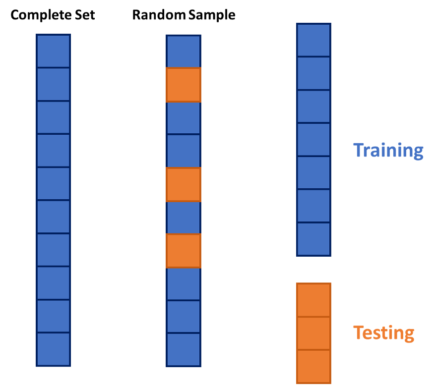
Before exploring any relationships between predictor variables and the target variable Sale_Price, we need to split our data set into training and testing pieces. Because models are prone to discovering small, spurious patterns on the data that is used to create them (the training data), we set aside the testing data to get a clear view of how they might perform on new data that the models have never seen before.

Code

library(tidyverse)

ames <- ames %>% mutate(id = row_number())

set.seed(4321)

training <- ames %>% sample_frac(0.7)
testing <- anti_join(ames, training, by = 'id')

This split is done randomly so that the testing data set will approximate an honest assessment of how the model will perform in a real world setting. A visual representation of this is below:

Splitting into Training and Testing Data

However, in the world of machine learning, we have a lot of aspects of a model that we need to “tune” or adjust to make our models more predictive. We can not perform this on the training data alone as it would lead to over-fitting (predicting too well) the training data and no longer generalizable. We could split the training data set again into a training and validation data set where the validation data set is what we “tune” our models on. The downside of this approach is that we will tend to start over-fitting the validation data set.

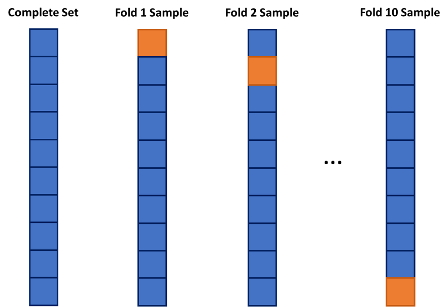
One approach to dealing with this is to use cross-validation. The idea of cross-validation is to divide your data set into k equally sized groups - called folds or samples. You leave one of the groups aside while building a model on the rest. You repeat this process of leaving one of the k folds out while building a model on the rest until each of the k folds has been left out once. We can evaluate a model by averaging the models’ effectiveness across all of the iterations. This process is highlighted below:

10-fold Cross-Validation Example

After initial exploration of our data set (not shown here) we are limiting down the variables to the following:

Code

training <- training %>% 
  select(Sale_Price,
         Bedroom_AbvGr,
         Year_Built,
         Mo_Sold,
         Lot_Area,
         Street,
         Central_Air,
         First_Flr_SF,
         Second_Flr_SF,
         Full_Bath,
         Half_Bath,
         Fireplaces,
         Garage_Area,
         Gr_Liv_Area, 
         TotRms_AbvGrd)

Model Selection

Although we will not cover the details behind linear and logistic regression here, we will see how cross-validation and model tuning concepts from machine learning can apply to these more classical statistical, linear models. For example, which variables should you drop from your model? This is a common question for all modeling, but especially generalized linear models. In this section we will cover a popular variable selection technique - stepwise regression, but from a machine learning standpoint.

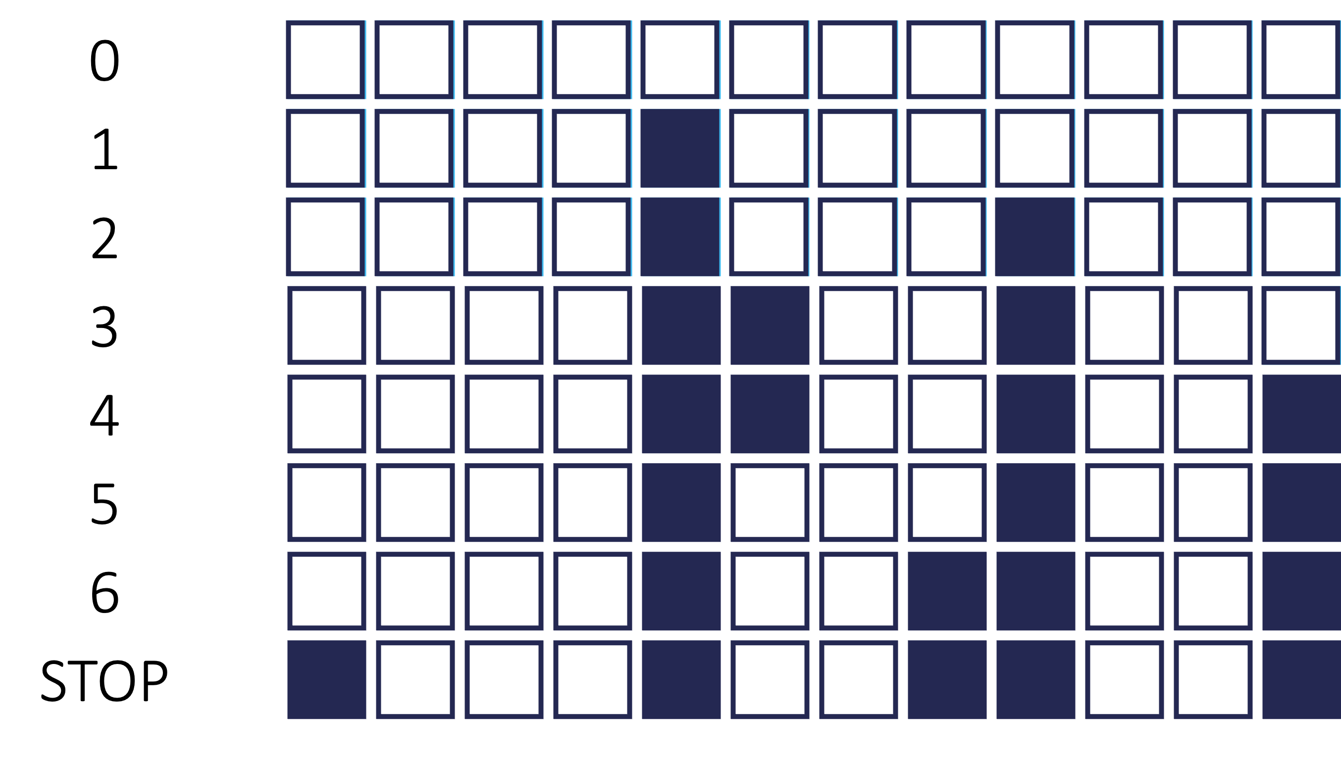
Stepwise regression techniques involve the three common methods:

1. Forward Selection
2. Backward Selection
3. Stepwise Selection

These techniques add or remove (depending the technique) one variable at a time from your regression model to try and “improve” the model. There are a variety of different selection criteria to use to add or remove variables from a logistic regression. Two common approaches are to use either p-values or one of the pair of AIC/BIC. The visual below shows an example of stepwise selection:

Stepwise Selection

However, from a machine learning standpoint, each step of the process is not evaluated on the training data, but on the cross-validation data sets. The model with the best average mean square error (MSE) in cross-validation is the one that moves on to the next step of the stepwise regression.

What we do with the results from this also differs depending on your background - the statistical/classical approach and the machine learning approach.

The more statistical and classical view would use validation to evaluate which model is “best” at each step of the process. The final model from the process contains the variables you want to keep in your model from that point going forward. To score a final test data set, you would combine the training and validation sets and then build a model with only the variables in the final step of the selection process. The coefficients on these variables might vary slightly because of the combining of the training and validation data sets.

The more machine learning approach is slightly different. You still use the validation to evaluate which model is “best” at each step in the process. However, instead of taking the variables in the final step of the process as the final variables to use, we look at the number of variables in the final step of the process as what has been optimized. To score a final test data set, you would combine the training and validation sets and then build a model with the same number of variables in the final process, but the variables don’t need to be the same as the ones in the final step of the process. The variables might be different because of the combining of the training and validation data sets.

Let’s see how to do this in each of our softwares!

R

Instead of using the traditional step function in R, we will be using the train function from the caret package to pull off stepwise regression with cross-validation. Inside of the train function we input the formula we want to predict the Sale_Price variable. Here we will use all of the other variables in the training data set (data = training option) by using the ~ . in our formula. The method = leapBackward option uses backward selection. The tuneGrid option controls what aspects of the model we are tuning to pick the best model. In stepwise selection the only tuning we can do is on the number of variables (nvmax = 1:14) which can be anything from 1 variable all the way to the max number of variables in our data set, 14. The trControl = trainControl(method = 'cv', number = '10') option makes the modeling process use 10-fold cross-validation for the model selection in each step of the process.

Code

library(caret)

set.seed(9876)

step.model <- caret::train(Sale_Price ~ ., data = training,
                    method = "leapBackward", 
                    tuneGrid = data.frame(nvmax = 1:14), 
                    trControl = trainControl(method = 'cv',
                                             number = 10))

Let’s explore the results from this backward selection through cross-validation. The results element of the model object shows the results from each step in the backward selection. The bestTune element shows the best values of the tuning variable (nvmax in this model).

Code

step.model$results

   nvmax     RMSE  Rsquared      MAE   RMSESD RsquaredSD    MAESD
1      1 61611.97 0.3942384 45180.98 5472.666 0.05620948 2526.312
2      2 49940.14 0.6074530 34262.71 7925.632 0.09929920 3450.872
3      3 42271.12 0.7153532 28108.76 7112.714 0.07760796 2655.431
4      4 41519.38 0.7274272 27291.26 7807.909 0.08250703 2626.796
5      5 39709.65 0.7505967 26396.47 7761.820 0.08026905 2621.732
6      6 39293.66 0.7556266 26266.02 7486.423 0.07609118 2547.016
7      7 39403.58 0.7542579 26256.86 7471.045 0.07604703 2553.544
8      8 39436.99 0.7538030 26265.14 7447.858 0.07528998 2562.365
9      9 39547.27 0.7525961 26324.07 7624.466 0.07703777 2651.493
10    10 39466.09 0.7536853 26281.15 7644.350 0.07719334 2660.940
11    11 39395.64 0.7546030 26253.80 7674.807 0.07729593 2706.320
12    12 39344.06 0.7552931 26195.33 7685.764 0.07737416 2753.871
13    13 39340.86 0.7553046 26182.74 7675.699 0.07725826 2737.195
14    14 39347.25 0.7553214 26190.40 7671.560 0.07724606 2724.610

Code

step.model$bestTune

  nvmax
6     6

For this model, the backward selection with 6 variables had the lowest MSE. Which variables were in this final model can be attained with the summary function on the finalModel element.

Code

summary(step.model$finalModel)

Subset selection object
14 Variables  (and intercept)
              Forced in Forced out
Bedroom_AbvGr     FALSE      FALSE
Year_Built        FALSE      FALSE
Mo_Sold           FALSE      FALSE
Lot_Area          FALSE      FALSE
StreetPave        FALSE      FALSE
Central_AirY      FALSE      FALSE
First_Flr_SF      FALSE      FALSE
Second_Flr_SF     FALSE      FALSE
Full_Bath         FALSE      FALSE
Half_Bath         FALSE      FALSE
Fireplaces        FALSE      FALSE
Garage_Area       FALSE      FALSE
Gr_Liv_Area       FALSE      FALSE
TotRms_AbvGrd     FALSE      FALSE
1 subsets of each size up to 6
Selection Algorithm: backward
         Bedroom_AbvGr Year_Built Mo_Sold Lot_Area StreetPave Central_AirY
1  ( 1 ) " "           " "        " "     " "      " "        " "         
2  ( 1 ) " "           " "        " "     " "      " "        " "         
3  ( 1 ) " "           "*"        " "     " "      " "        " "         
4  ( 1 ) " "           "*"        " "     " "      " "        " "         
5  ( 1 ) "*"           "*"        " "     " "      " "        " "         
6  ( 1 ) "*"           "*"        " "     " "      " "        " "         
         First_Flr_SF Second_Flr_SF Full_Bath Half_Bath Fireplaces Garage_Area
1  ( 1 ) "*"          " "           " "       " "       " "        " "        
2  ( 1 ) "*"          "*"           " "       " "       " "        " "        
3  ( 1 ) "*"          "*"           " "       " "       " "        " "        
4  ( 1 ) "*"          "*"           " "       " "       " "        "*"        
5  ( 1 ) "*"          "*"           " "       " "       " "        "*"        
6  ( 1 ) "*"          "*"           " "       " "       "*"        "*"        
         Gr_Liv_Area TotRms_AbvGrd
1  ( 1 ) " "         " "          
2  ( 1 ) " "         " "          
3  ( 1 ) " "         " "          
4  ( 1 ) " "         " "          
5  ( 1 ) " "         " "          
6  ( 1 ) " "         " "          

The six variables in the final model shown above are First_Flr_SF, Second_Flr_SF, Year_Built, Garage_Area, Bedroom_AbvGr, and Fireplaces.

The classical view of model building would use these 6 variables built on the entire training set with no cross-validation as shown below:

Code

final.model1 <- glm(Sale_Price ~ First_Flr_SF + 
                                 Second_Flr_SF + 
                                 Year_Built + 
                                 Garage_Area + 
                                 Bedroom_AbvGr +
                                 Fireplaces,
                    data = training)

summary(final.model1)

Call:
glm(formula = Sale_Price ~ First_Flr_SF + Second_Flr_SF + Year_Built + 
    Garage_Area + Bedroom_AbvGr + Fireplaces, data = training)

Coefficients:
                Estimate Std. Error t value Pr(>|t|)    
(Intercept)   -1.407e+06  6.439e+04 -21.852  < 2e-16 ***
First_Flr_SF   1.128e+02  3.236e+00  34.871  < 2e-16 ***
Second_Flr_SF  8.252e+01  2.812e+00  29.342  < 2e-16 ***
Year_Built     7.256e+02  3.306e+01  21.945  < 2e-16 ***
Garage_Area    6.012e+01  5.366e+00  11.203  < 2e-16 ***
Bedroom_AbvGr -1.265e+04  1.317e+03  -9.607  < 2e-16 ***
Fireplaces     1.113e+04  1.555e+03   7.157 1.14e-12 ***
---
Signif. codes:  0 '***' 0.001 '**' 0.01 '*' 0.05 '.' 0.1 ' ' 1

(Dispersion parameter for gaussian family taken to be 1561167099)

    Null deviance: 1.275e+13  on 2050  degrees of freedom
Residual deviance: 3.191e+12  on 2044  degrees of freedom
AIC: 49246

Number of Fisher Scoring iterations: 2

The machine learning view would go through a backward selection process on the entire training set with no cross-validation and just pick the model with the “best” 6 variables as shown below. Notice that there are 5 variables of the six that are the same as the classical approach, but one that is different - Gr_Liv_Area.

Code

empty.model <- glm(Sale_Price ~ 1, data = training)
full.model <- glm(Sale_Price ~ ., data = training)

final.model2 <- step(empty.model, scope = list(lower = formula(empty.model),
                                               upper = formula(full.model)),
                     direction = "both", steps = 6, trace = FALSE)

summary(final.model2)

Call:
glm(formula = Sale_Price ~ Gr_Liv_Area + Year_Built + First_Flr_SF + 
    Garage_Area + Bedroom_AbvGr + Fireplaces, data = training)

Coefficients:
                Estimate Std. Error t value Pr(>|t|)    
(Intercept)   -1.441e+06  6.451e+04 -22.343  < 2e-16 ***
Gr_Liv_Area    8.116e+01  2.790e+00  29.086  < 2e-16 ***
Year_Built     7.433e+02  3.313e+01  22.438  < 2e-16 ***
First_Flr_SF   3.053e+01  2.944e+00  10.370  < 2e-16 ***
Garage_Area    6.110e+01  5.373e+00  11.372  < 2e-16 ***
Bedroom_AbvGr -1.258e+04  1.322e+03  -9.518  < 2e-16 ***
Fireplaces     1.138e+04  1.558e+03   7.305 3.95e-13 ***
---
Signif. codes:  0 '***' 0.001 '**' 0.01 '*' 0.05 '.' 0.1 ' ' 1

(Dispersion parameter for gaussian family taken to be 1569252272)

    Null deviance: 1.2750e+13  on 2050  degrees of freedom
Residual deviance: 3.2076e+12  on 2044  degrees of freedom
AIC: 49257

Number of Fisher Scoring iterations: 2

Python

We first need to get our training data set prepared for modeling in Python. We can use the get_dummies function from pandas to turn our categorical variables of Street and Central_Air into dummy variable (one-hot encoding) representations. The next step is creating two objects, one for the target variable (called y_train) and one for all the predictor variables (X_train).

Code

import pandas as pd

train_dummy = pd.get_dummies(training, columns = ['Street', 'Central_Air'])

print(train_dummy)

      Sale_Price  Bedroom_AbvGr  ...  Central_Air_N  Central_Air_Y
0         274000              3  ...              0              1
1          75200              2  ...              0              1
2         329900              4  ...              0              1
3         145400              3  ...              0              1
4         108000              2  ...              0              1
...          ...            ...  ...            ...            ...
2046      192000              2  ...              0              1
2047      160200              2  ...              0              1
2048      171500              2  ...              0              1
2049      151500              3  ...              0              1
2050      156500              4  ...              0              1

[2051 rows x 17 columns]

Code

y_train = train_dummy['Sale_Price']

X_train = train_dummy.loc[:, train_dummy.columns != 'Sale_Price']

With the data now in a format for modeling, we use the LinearRegression function from sklearn as an input to the SequentialFeatureSelector function. We set the n_features_to_select = "auto" option to not limit how many variables the model can choose. The direction = "backward" option specifies the backward selection process. To get the best model according to cross-validation MSE we use the scoring = "neg_mean_squared_error", cv = 10 options.

Code

from sklearn.feature_selection import SequentialFeatureSelector
from sklearn.linear_model import LinearRegression
from sklearn.model_selection import KFold

lm = LinearRegression()

model_cv = SequentialFeatureSelector(lm, n_features_to_select = "auto", direction = "backward", scoring = "neg_mean_squared_error", cv = 10)

model_cv.fit(X_train, y_train)

SequentialFeatureSelector(cv=10, direction='backward',
                          estimator=LinearRegression(),
                          n_features_to_select='auto',
                          scoring='neg_mean_squared_error')

In a Jupyter environment, please rerun this cell to show the HTML representation or trust the notebook.
On GitHub, the HTML representation is unable to render, please try loading this page with nbviewer.org.

To get the variables from this model we use the get_feature_names_out() element from model object.

Code

model_cv.get_feature_names_out()

array(['Bedroom_AbvGr', 'Year_Built', 'Mo_Sold', 'Lot_Area',
       'First_Flr_SF', 'Second_Flr_SF', 'Fireplaces', 'Garage_Area'],
      dtype=object)

For this model, the backward selection with 8 variables had the lowest MSE. The 8 variables are Bedroom_AbvGr, Year_Built, Mo_Sold, Lot_Area, First_Flr_SF, Second_Flr_SF, Fireplaces, and Garage_Area.

The classical view of model building would use these 8 variables built on the entire training set with no cross-validation as shown below:

Code

import statsmodels.formula.api as smf

final_model1 = smf.ols("Sale_Price ~ Bedroom_AbvGr + Year_Built + Mo_Sold + Lot_Area + First_Flr_SF + Second_Flr_SF + Fireplaces + Garage_Area", data = training).fit()

final_model1.summary()

OLS Regression Results

Dep. Variable:	Sale_Price	R-squared:	0.751
Model:	OLS	Adj. R-squared:	0.750
Method:	Least Squares	F-statistic:	770.2
Date:	Mon, 23 Oct 2023	Prob (F-statistic):	0.00
Time:	16:02:22	Log-Likelihood:	-24610.
No. Observations:	2051	AIC:	4.924e+04
Df Residuals:	2042	BIC:	4.929e+04
Df Model:	8
Covariance Type:	nonrobust

	coef	std err	t	P>|t|	[0.025	0.975]
Intercept	-1.424e+06	6.48e+04	-21.973	0.000	-1.55e+06	-1.3e+06
Bedroom_AbvGr	-1.265e+04	1318.042	-9.597	0.000	-1.52e+04	-1.01e+04
Year_Built	735.8717	33.253	22.130	0.000	670.659	801.084
Mo_Sold	-620.2853	322.729	-1.922	0.055	-1253.199	12.628
Lot_Area	0.3102	0.115	2.703	0.007	0.085	0.535
First_Flr_SF	111.2926	3.289	33.838	0.000	104.842	117.743
Second_Flr_SF	82.3112	2.807	29.324	0.000	76.806	87.816
Fireplaces	1.071e+04	1562.548	6.853	0.000	7643.160	1.38e+04
Garage_Area	59.1374	5.375	11.001	0.000	48.595	69.679

Omnibus:	634.179	Durbin-Watson:	1.956
Prob(Omnibus):	0.000	Jarque-Bera (JB):	40998.546
Skew:	-0.577	Prob(JB):	0.00
Kurtosis:	24.873	Cond. No.	9.82e+05

Notes:
[1] Standard Errors assume that the covariance matrix of the errors is correctly specified.
[2] The condition number is large, 9.82e+05. This might indicate that there are
strong multicollinearity or other numerical problems.

The machine learning view would go through a backward selection process on the entire training set with no cross-validation and just pick the model with the “best” 8 variables as shown below. Notice that there are 5 variables of the six that are the same as the classical approach, but one that is different - Central_Air_N.

Code

final_model2 = SequentialFeatureSelector(lm, n_features_to_select = 8, direction = "backward", scoring = "neg_mean_squared_error")

final_model2.fit(X_train, y_train)

SequentialFeatureSelector(direction='backward', estimator=LinearRegression(),
                          n_features_to_select=8,
                          scoring='neg_mean_squared_error')

In a Jupyter environment, please rerun this cell to show the HTML representation or trust the notebook.
On GitHub, the HTML representation is unable to render, please try loading this page with nbviewer.org.

Code

final_model2.get_feature_names_out()

array(['Bedroom_AbvGr', 'Year_Built', 'Mo_Sold', 'First_Flr_SF',
       'Second_Flr_SF', 'Fireplaces', 'Garage_Area', 'Central_Air_N'],
      dtype=object)

Regularization

Linear regression is a great initial approach to take to model building. In fact, in the realm of statistical models, linear regression (calculated by ordinary least squares) is the best linear unbiased estimator. The two key pieces to that previous statement are “best” and “unbiased.”

What does it mean to be unbiased? Each of the sample coefficients (\(\hat{\beta}\)’s) in the regression model are estimates of the true coefficients. These sample coefficients have sampling distributions - specifically, normally distributed sampling distributions. The mean of the sampling distribution of \(\hat{\beta}_j\) is the true (known) coefficient \(\beta_j\). This means the coefficient is unbiased.

What does it mean to be best? IF the assumptions of ordinary least squares are met fully, then the sampling distributions of the coefficients in the model have the minimum variance of all unbiased estimators.

These two things combined seem like what we want in a model - estimating what we want (unbiased) and doing it in a way that has the minimum amount of variation (best among the unbiased). Again, these rely on the assumptions of linear regression holding true. Another approach to regression would be to use regularized regression instead as a different approach to building the model.

As the number of variables in a linear regression model increase, the chances of having a model that meets all of the assumptions starts to diminish. Multicollinearity can pose a large problem with bigger regression models. The coefficients of a linear regression vary widely in the presence of multicollinearity. These variations lead to over-fitting of a regression model. More formally, these models have higher variance than desired. In those scenarios, moving out of the realm of unbiased estimates may provide a lower variance in the model, even though the model is no longer unbiased as described above. We wouldn’t want to be too biased, but some small degree of bias might improve the model’s fit overall and even lead to better predictions at the cost of a lack of interpretability.

Another potential problem for linear regression is when we have more variables than observations in our data set. This is a common problem in the space of genetic modeling. In this scenario, the ordinary least squares approach leads to multiple solutions instead of just one. Unfortunately, most of these infinite solutions over-fit the problem at hand anyway.

Regularized (or penalized or shrinkage) regression techniques potentially alleviate these problems. Regularized regression puts constraints on the estimated coefficients in our model and shrink these estimates to zero. This helps reduce the variation in the coefficients (improving the variance of the model), but at the cost of biasing the coefficients. The specific constraints that are put on the regression inform the three common approaches - ridge regression, LASSO, and elastic nets.

Penalties in Models

In ordinary least squares linear regression, we minimize the sum of the squared residuals (or errors).

\[ min(\sum_{i=1}^n(y_i - \hat{y}_i)^2) = min(SSE) \]

In regularized regression, however, we add a penalty term to the \(SSE\) as follows:

\[ min(\sum_{i=1}^n(y_i - \hat{y}_i)^2 + Penalty) = min(SSE + Penalty) \]

As mentioned above, the penalties we choose constrain the estimated coefficients in our model and shrink these estimates to zero. Different penalties have different effects on the estimated coefficients. Two common approaches to adding penalties are the ridge and LASSO approaches. The elastic net approach is a combination of these two. Let’s explore each of these in further detail.

Ridge Regression

Ridge regression adds what is commonly referred to as an “\(L_2\)” penalty:

\[ min(\sum_{i=1}^n(y_i - \hat{y}_i)^2 + \lambda \sum_{j=1}^p \hat{\beta}^2_j) = min(SSE + \lambda \sum_{j=1}^p \hat{\beta}^2_j) \]

This penalty is controlled by the tuning parameter \(\lambda\). If \(\lambda = 0\), then we have typical OLS linear regression. However, as \(\lambda \rightarrow \infty\), the coefficients in the model shrink to zero. This makes intuitive sense. Since the estimated coefficients, \(\hat{\beta}_j\)’s, are the only thing changing to minimize this equation, then as \(\lambda \rightarrow \infty\), the equation is best minimized by forcing the coefficients to be smaller and smaller. We will see how to optimize this penalty term in a later section.

LASSO

Least absolute shrinkage and selection operator (LASSO) regression adds what is commonly referred to as an “\(L_1\)” penalty:

\[ min(\sum_{i=1}^n(y_i - \hat{y}_i)^2 + \lambda \sum_{j=1}^p |\hat{\beta}_j|) = min(SSE + \lambda \sum_{j=1}^p |\hat{\beta}_j|) \]

This penalty is controlled by the tuning parameter \(\lambda\). If \(\lambda = 0\), then we have typical OLS linear regression. However, as \(\lambda \rightarrow \infty\), the coefficients in the model shrink to zero. This makes intuitive sense. Since the estimated coefficients, \(\hat{\beta}_j\)’s, are the only thing changing to minimize this equation, then as \(\lambda \rightarrow \infty\), the equation is best minimized by forcing the coefficients to be smaller and smaller. We will see how to optimize this penalty term in a later section.

However, unlike ridge regression that has the coefficient estimates approach zero asymptotically, in LASSO regression the coefficients can actually equal zero. This may not be as intuitive when initially looking at the penalty terms themselves. It becomes easier to see when dealing with the solutions to the coefficient estimates. Without going into too much mathematical detail, this is done by taking the derivative of the minimization function (objective function) and setting it equal to zero. From there we can determine the optimal solution for the estimated coefficients. In OLS regression the estimates for the coefficients can be shown to equal the following (in matrix form):

\[ \hat{\beta} = (X^TX)^{-1}X^TY \]

This changes in the presence of penalty terms. For ridge regression, the solution becomes the following:

\[ \hat{\beta} = (X^TX + \lambda I)^{-1}X^TY \]

There is no value for \(\lambda\) that can force the coefficients to be zero by itself. Therefore, unless the data makes the coefficient zero, the penalty term can only force the estimated coefficient to zero asymptotically as \(\lambda \rightarrow \infty\).

However, for LASSO, the solution becomes the following:

\[ \hat{\beta} = (X^TX)^{-1}(X^TY - \lambda I) \]

Notice the distinct difference here. In this scenario, there is a possible penalty value (\(\lambda = X^TY\)) that will force the estimated coefficients to equal zero. There is some benefit to this. This makes LASSO also function as a variable selection criteria as well.

Elastic Net

Which approach is better, ridge or LASSO? Both have advantages and disadvantages. LASSO performs variable selection while ridge keeps all variables in the model. However, reducing the number of variables might impact minimum error. Also, if you have two correlated variables, which one LASSO chooses to zero out is relatively arbitrary to the context of the problem.

Elastic nets were designed to take advantage of both penalty approaches. In elastic nets, we are using both penalties in the minimization:

\[ min(SSE + \lambda_1 \sum_{j=1}^p |\hat{\beta}_j| + \lambda_2 \sum_{j=1}^p \hat{\beta}^2_j) \]

In R, the glmnet function takes a slightly different approach to the elastic net implementation with the following:

\[ min(SSE + \lambda[ \alpha \sum_{j=1}^p |\hat{\beta}_j| + (1-\alpha) \sum_{j=1}^p \hat{\beta}^2_j]) \]

R still has one penalty \(\lambda\), however, it includes the \(\alpha\) parameter to balance between the two penalty terms. Any value in between zero and one will provide an elastic net.

Let’s see how to build these models in each of our softwares!

R

Let’s build a regularized regression for our Ames dataset. Instead of trying to decide ahead of time whether a ridge, LASSO, or Elastic net regression would be better for our data, we will let that balance be part of the tuning for our model. We will use the same train function as before. Now we will use the method = "glmnet" option to build a regularized regression. Inside of our tuneGrid option we have multiple things to tune. The expand.grid function will fill in all of the combinations of values we want to tune. The .alpha = option is looking at the balance of the two penalties as described above. We will test values between 0 (ridge regression) to 1 (LASSO regression) by values of 0.05. We will also test different levels of the \(\lambda\) penalty using the .lambda = option. The trControl option stays the same to allow us to tune these models using 10-fold cross-validation.

Code

set.seed(5)

en.model <- caret::train(Sale_Price ~ ., data = training,
                  method = "glmnet", 
                  tuneGrid = expand.grid(.alpha = seq(0,1, by = 0.05),
                                         .lambda = seq(100,60000, by = 1000)), 
                  trControl = trainControl(method = 'cv', 
                                             number = 10))

Warning in nominalTrainWorkflow(x = x, y = y, wts = weights, info = trainInfo,
: There were missing values in resampled performance measures.

Code

en.model$bestTune

    alpha lambda
601   0.5    100

As we can see at the bottom of the output above with the bestTune option, the optimal model has an \(\alpha = 0.5\) and \(\lambda = 100\).

R has an ability to do more fine tuned optimization of the \(\lambda\) parameter outside of the train function by using the glmnet function and package directly. However, the glmnet function doesn’t have the ability to optimize the \(\alpha\) parameter like the train function.

In R, the cv.glmnet function will automatically implement a 10-fold CV (by default, but can be adjusted through options) to help evaluate and optimize the \(\lambda\) values for our regularized regression models at a finer tune than the train function of caret.

We will build an elastic net with \(\alpha = 0.5\) that we determined from the previous tuning. To build a model with the glmnet package we need separate data matrices for our predictors and our target variable. First, we use the model.matrix function will create any categorical dummy variables needed. We also isolate the target variable into its own vector. From there we use the glmnet function with the x = option where we specify the predictor model matrix and the y = option where we specify the target variable. The alpha = 0.5 option specifies that an elastic net will be used since it is between zero and one. The plot function allows us to see the impact of the penalty on the coefficients in the model.

Code

library(glmnet)

Loading required package: Matrix

Attaching package: 'Matrix'

The following objects are masked from 'package:tidyr':

    expand, pack, unpack

Loaded glmnet 4.1-7

Code

train_x <- model.matrix(Sale_Price ~ ., data = training)[, -1]
train_y <- training$Sale_Price

ames_en <- glmnet(x = train_x,  y = train_y,  alpha = 0.5)

plot(ames_en, xvar = "lambda")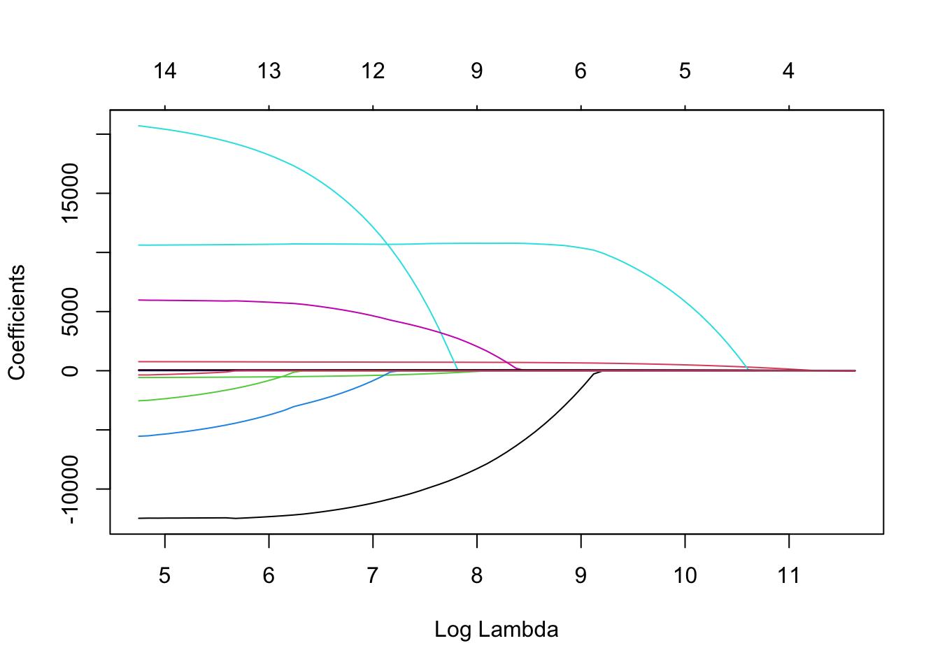

The glmnet function automatically standardizes the variables before fitting the regression model. This is important so that all of the variables are on the same scale before adjustments are made to the estimated coefficients. Even with this standardization we can see the large coefficient values for some of the variables. The top of the plot lists how many variables are in the model at each value of penalty. Notice as the penalty increases, the number of variables decreases as variables are forced to zero.

In R, the cv.glmnet function will automatically implement a 10-fold CV (by default, but can be adjusted through options) to help evaluate and optimize the \(\lambda\) values for our regularized regression models. The cv.glmnet function takes the same inputs as the glmnet function above. Again, we will use the plot function, but this time we get a different plot.

Code

set.seed(5)

ames_en_cv <- cv.glmnet(x = train_x,  y = train_y,  alpha = 0.5)

plot(ames_en_cv)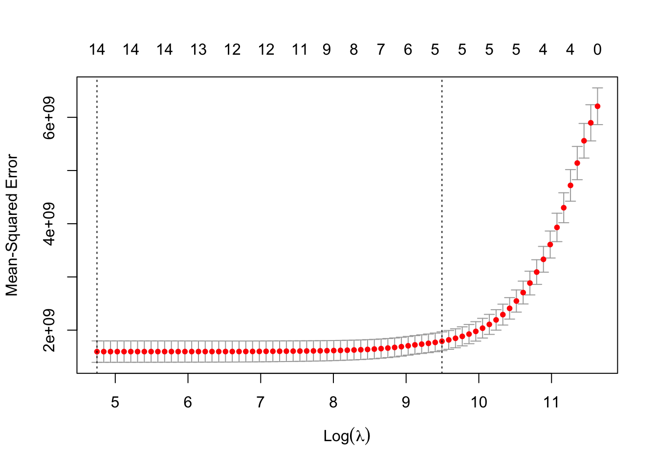

Code

ames_en_cv$lambda.min

[1] 115.4119

Code

ames_en_cv$lambda.1se

[1] 13269.57

The above plot shows the results from our cross-validation. Here the models are evaluated based on their mean-squared error (MSE). The MSE is defined as \(\frac{1}{n} \sum_{i=1}^n (y_i - \hat{y}_i)^2\). The \(\lambda\) value that minimizes the MSE is 115.4119 (with a \(\log(\lambda)\) = 4.75). This is highlighted by the first, vertical dashed line. The second vertical dashed line is the largest \(\lambda\) value that is one standard error above the minimum value. This value is especially useful in LASSO or elastic net regressions. The largest \(\lambda\) within one standard error would provide approximately the same MSE, but with a further reduction in the number of variables. Notice that to go from the first line to the second, the change in MSE is very small, but the reduction of variables is from 14 variables to around 5 variables.

Python

Let’s build a regularized regression for our Ames dataset. Instead of trying to decide ahead of time whether a ridge, LASSO, or Elastic net regression would be better for our data, we will let that balance be part of the tuning for our model. We will use the ElasticNetCV function from sklearn. We specify a 10-fold cross-validation using the cv =10 option. The l1ratio = option is looking at the balance of the two penalties as described above. We will test values between 0 (ridge regression) to 1 (LASSO regression) by values of 0.1. We will also test different levels of the \(\lambda\) penalty using the n_alphas = option where we specify that we want it to test 100 different values. The naming conventions in the options are a little different than the equations above, but the idea remains the same.

Code

from sklearn.linear_model import ElasticNetCV

en_model = ElasticNetCV(cv = 10, l1_ratio = [0.1, 0.2, 0.3, 0.4, 0.5, 0.6, 0.7, 0.8, 0.9], n_alphas = 100)

en_model.fit(X_train, y_train)

ElasticNetCV(cv=10, l1_ratio=[0.1, 0.2, 0.3, 0.4, 0.5, 0.6, 0.7, 0.8, 0.9])

In a Jupyter environment, please rerun this cell to show the HTML representation or trust the notebook.
On GitHub, the HTML representation is unable to render, please try loading this page with nbviewer.org.

Code

en_model.alpha_

181220.69508991155

Code

en_model.l1_ratio_

0.9

As we can see at the bottom of the output above by inspecting the alpha_ and l1_ratio elements, the optimal model has an \(\alpha = 0.9\) and \(\lambda = 181220.7\).

To view the impact of different values of the \(\lambda\) penalty on the elastic net model, we can use Python’s ElasticNet function. We will look at the impact on the coefficients across many different values of the penalty term (alpha = option in ElasticNet). Using the logspace function from numpy we can get 100 different values between 1 and 8 to visualize for the penalty. We just evaluate these in a for loop setting the l1_ratio to be 0.9 as we determined above. From there we build the plot.

Code

import numpy as np
from sklearn.linear_model import ElasticNet
from matplotlib import pyplot as plt
import seaborn as sns

n_alphas = 100
alphas3 = np.logspace(1, 8, n_alphas)

coefs3 = []
for a in alphas3:
    en = ElasticNet(alpha = a, l1_ratio=0.9)
    en.fit(X_train, y_train)
    coefs3.append(en.coef_)

ElasticNet(alpha=100000000.0, l1_ratio=0.9)

In a Jupyter environment, please rerun this cell to show the HTML representation or trust the notebook.
On GitHub, the HTML representation is unable to render, please try loading this page with nbviewer.org.

Code

    
plt.cla()
ax3 = plt.gca()

ax3.plot(alphas3, coefs3)
ax3.set_xscale("log")
plt.xlabel("alpha")
plt.ylabel("weights")
plt.title("ElasticNet coefficients as a function of the regularization")
plt.axis("tight")

(4.46683592150963, 223872113.8568338, -4198.359820212884, 3229.576658889914)

Code

plt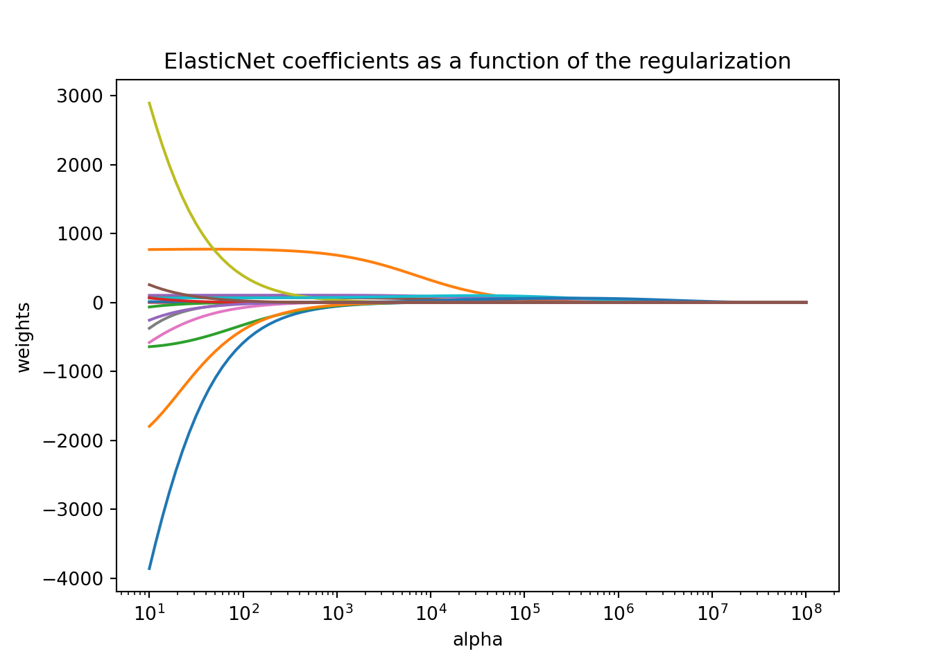.show()

The ElasticNet function automatically standardizes the variables before fitting the regression model. This is important so that all of the variables are on the same scale before adjustments are made to the estimated coefficients. Even with this standardization we can see the large coefficient values for some of the variables. Notice as the penalty increases, the number of variables decreases as variables are forced to zero.