Code
library(randomForest)

training.df <- as.data.frame(training)

set.seed(12345)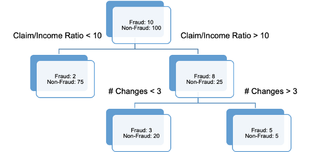
rf.ames <- randomForest(Sale_Price ~ ., data = training.df, ntree = 500, importance = TRUE)A decision tree can be used to predict either categorical or continuous variables. The tree is built by recursively splitting the data into successively purer subsets of data. The purity of a node is looking at how “homogeneous” the node is with respect to the target variable. These splits are done based on some condition:
Measurements of purity - Gini, entropy, misclassification error rate
\(\chi^2\) tests (CHAID)
Most trees use binary splits (only allows for two options each time a variable is chosen), but some algorithms will do more. Every possible split is evaluated by one of the metrics above and the best split is chosen. This process is repeated until no more splits meet the criteria.
Decision trees are great because they are very interpretable as you work down through the tree. However, if you are willing to forgo some of the interpretability, these trees can be ensembled to make better predictions.
This section will detail two common ensembling techniques - boosting and bagging - and the algorithms that derive from them.
Before understanding the concept of bagging, we need to know what a bootstrap sample is. A Bootstrap sample is a random sample of your data with replacement that are the same size as your original data set. By random chance, some of the observations will not be sampled. These observations are called out-of-bag observations. Three example bootstrap samples of 10 observations labelled 1 through 10 are listed below:
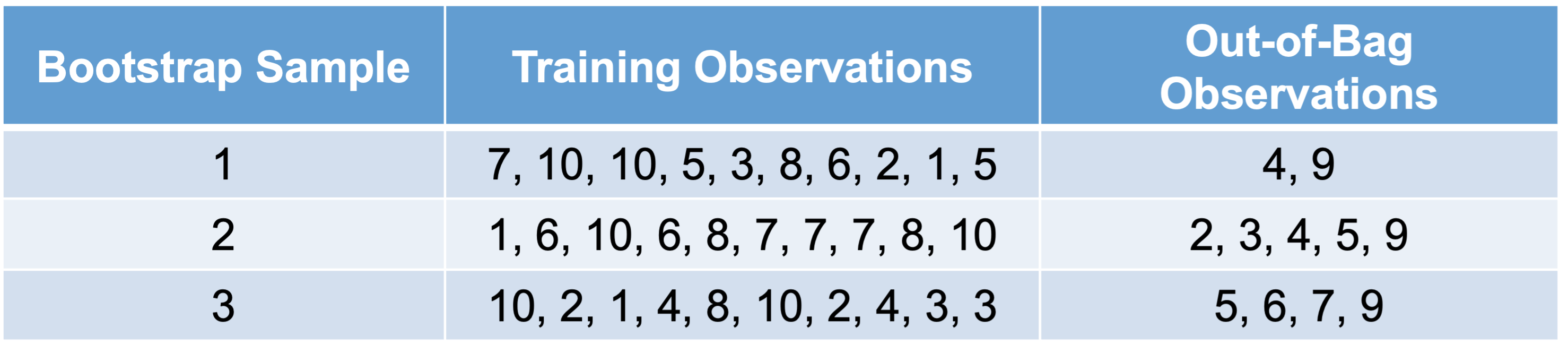
Mathematically, a bootstrap sample will contain approximately 63% of the observations in the data set. The sample size of the bootstrap sample is the same as the original data set, just some observations are repeated. Bootstrap samples are used in simulation to help develop confidence intervals of complicated forecasting techniques. Bootstrap samples are also used to ensemble models using different training data sets - called bagging.
Bootstrap aggregating (bagging) is where you take k bootstrap samples and create a model using each of the bootstrap samples as the training data set. This will build k different models. We will ensemble these k different models together.
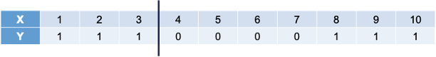
Let’s work through an example to see the potential value. The following 10 observations have the values of X and Y shown in the following table:

We will build a decision stump (a decision tree with only one split). From building a decision stump, the best accuracy is obtained by making the split at either 3.5 or 7.5. Either of these splits would lead to an accuracy of predicting Y at 70%. For example, let’s use the split at 3.5. That would mean we think everything above 3.5 is a 0 and everything below 3.5 is a 1. We would get observations 1, 2, and 3 all correct. However, since everything above 3.5 is considered a 0, we would only get observations 4, 5, 6, and 7 correct on that piece - missing observations 8, 9, and 10.
To try and make this prediction better we will do the following:
The following is the 10 bootstrap samples with their optimal splits. Remember, these bootstrap samples will not contain all of the observations in the original data set.
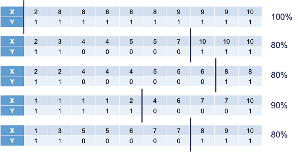
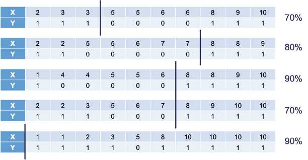
Some of these samples contain only one value of the target variable and so the predictions are the same for that bootstrap sample. However, we will use the optimal cut-offs from each of those samples to predict 1’s and 0’s for the original data set as shown in the table below:
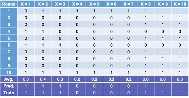
The table above has one row for each of the predictions from the 10 bootstrap samples. We can average these predictions of 1’s and 0’s together for each observation to get the average row near the bottom.
Let’s take a cut-off of 0.25 from our average values from the 1 and 0 predictions from each bootstrap sample. That would mean anything above 0.25 in the average row would be predicted as a 1 while everything below would be predicted as a 0. Based on those predictions (the Pred. row above) we get a perfect prediction compared to the true values of Y from our original data set.
In summary, bagging improves generalization error on models with high variance (simple tree-based models for example). If base classifier is stable (not suffering from high variance), then bagging can actually make predictions worse! Bagging does not focus on particular observations in the training data set (unlike boosting which is covered below).
Random forests are ensembles of decision trees (similar to the bagging example from above). Ensembles of decision trees work best when they find different patterns in the data. However, bagging tends to create trees that pick up the same pattern.
Random forests get around this correlation between trees by not only using bootstrapped samples, but also uses subsets of variables for each split and unpruned decision trees. For these unpruned trees, with a classification target it goes all the way until each unique observation is left in its own leaf. With regression trees the unpruned trees will continue until 5 observations are left per leaf. The results from all of these trees are ensembled together into one voting system. There are many choices of parameters to tune:
Let’s see random forests in each of our softwares!
Let’s build a random forest with our Ames housing data set. For the randomForest function, we need our data set in a data frame - using the as.data.frame function. The randomForest package with the randomForest function is one way to build random forests in R. Similar to other functions, we have a formula as well as a data = option. We also have a ntree option where we will start by looking at 500 decision trees in the ensemble model. The importance = TRUE option gives the variable importance from the random forest.
library(randomForest)
training.df <- as.data.frame(training)
set.seed(12345)
rf.ames <- randomForest(Sale_Price ~ ., data = training.df, ntree = 500, importance = TRUE)Unlike some of the previous models where there was a summary of the model we could look at, random forests are different. Since it is an ensemble of 500 different models, we do not have that ability. However, there are some things we can look at with this function. We will use the plot function to see how the number of trees increasing improves the MSE of the model.
plot(rf.ames, main = "Number of Trees Compared to MSE")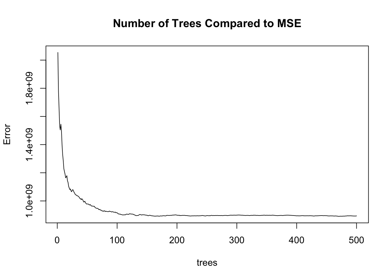
We can see from the plot above that the MSE of the whole training set seems to level off around 250 trees. Beyond that, adding more trees only increases the computation time, but not the predictive power of the model.
We can also use the varImpPlot function to plot the variables by importance in the random forest. The sort = TRUE option sorts the variables from best to worst, while the n.var option controls how many variables are shown. Every variable is in the random forest to some degree. The importance function will list the variables’ actual values of importance instead of just plotting them.
varImpPlot(rf.ames,
           sort = TRUE,
           n.var = 10,
           main = "Top 10 - Variable Importance")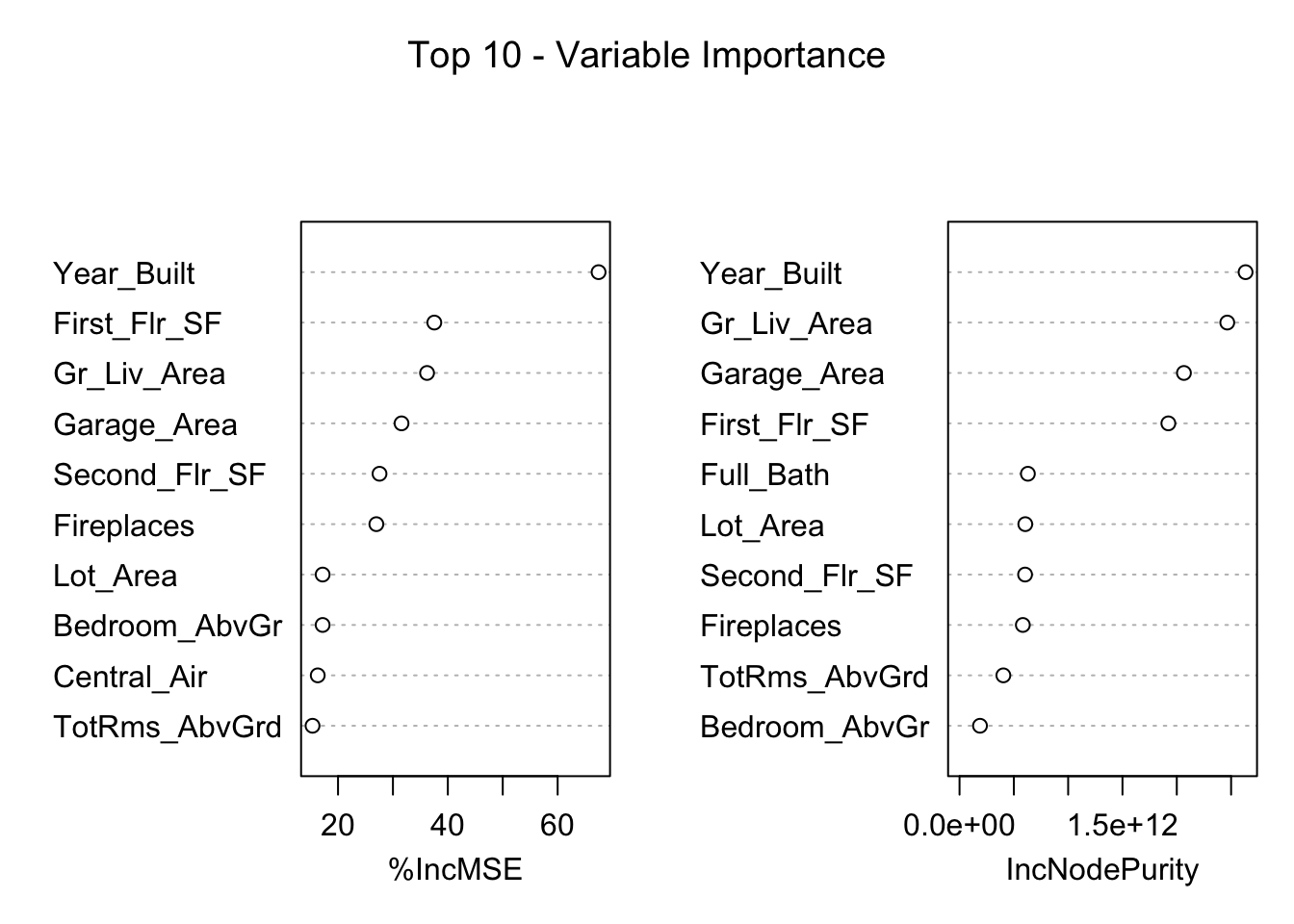
importance(rf.ames) %IncMSE IncNodePurity
Bedroom_AbvGr 17.196874 1.883174e+11
Year_Built 67.454195 2.633279e+12
Mo_Sold 2.784443 1.851229e+11
Lot_Area 17.197520 6.052979e+11
Street 5.653205 4.434557e+09
Central_Air 16.304359 9.601244e+10
First_Flr_SF 37.534894 1.922377e+12
Second_Flr_SF 27.556173 6.032976e+11
Full_Bath 14.814608 6.292031e+11
Half_Bath 13.736134 1.042685e+11
Fireplaces 26.979404 5.827696e+11
Garage_Area 31.565869 2.065680e+12
Gr_Liv_Area 36.214537 2.464645e+12
TotRms_AbvGrd 15.357145 4.033601e+11The left-hand plot above (and left hand column in the table) shows the percentage increase in MSE when the variable is “excluded” from the model. In other words, how much worse is the model when that variable’s impact is no longer there. The variables that make the model the worst by the most will be high in importance. The variable isn’t actually removed from the modeling process, but the values are permuted (randomly shuffled around) to remove the impact of that variable. By this metric (called permutation importance), Year-Built is by far the most important variable.
The right-hand plot above (and right hand column in the table) shows the increase in purity in the nodes of the tree - essentially measuring how much each variable improves the purity of the model when it is added. Again, Year_Built is at the top of the list.
Let’s build a random forest with our Ames housing data set. We will use the RandomForestRegressor function from the sklearn.ensemble package. Similar to other Python functions we have used, we need the training predictor variables in one object and the target variable in another. The option to define how many decision trees are in the ensemble is n_estimators.
from sklearn.ensemble import RandomForestRegressor

rf_ames = RandomForestRegressor(n_estimators = 100,
                                  random_state = 12345,
                                  oob_score = True)

rf_ames.fit(X_train, y_train)
RandomForestRegressor(oob_score=True, random_state=12345)In a Jupyter environment, please rerun this cell to show the HTML representation or trust the notebook.
RandomForestRegressor(oob_score=True, random_state=12345)
The random_state option helps set the seed for the function to make the results repeatable. The oob_score = True option calculates the out-of-bag score for the model chosen for comparisons to other models of different sizes. Let’s view that out-of-bag score with call of the oos_score_ element from the model object.
rf_ames.oob_score_0.8551822614732704We can also use the feature_importance_ element from the random forest model to plot the variables by importance in the random forest. Here we create a pd.Series object with the feature_importances_ element as well as the feature_names_in_ element as the index. Every variable is in the random forest to some degree. From there we just use a plot.bar function from matplotlib.
from matplotlib import pyplot as plt
import seaborn as sns

forest_importances = pd.Series(rf_ames.feature_importances_, index = rf_ames.feature_names_in_)

fig, ax = plt.subplots()
forest_importances.plot.bar(ax = ax)
ax.set_title("Feature importances")
ax.set_ylabel("Mean decrease in impurity")
fig.tight_layout()

plt.show()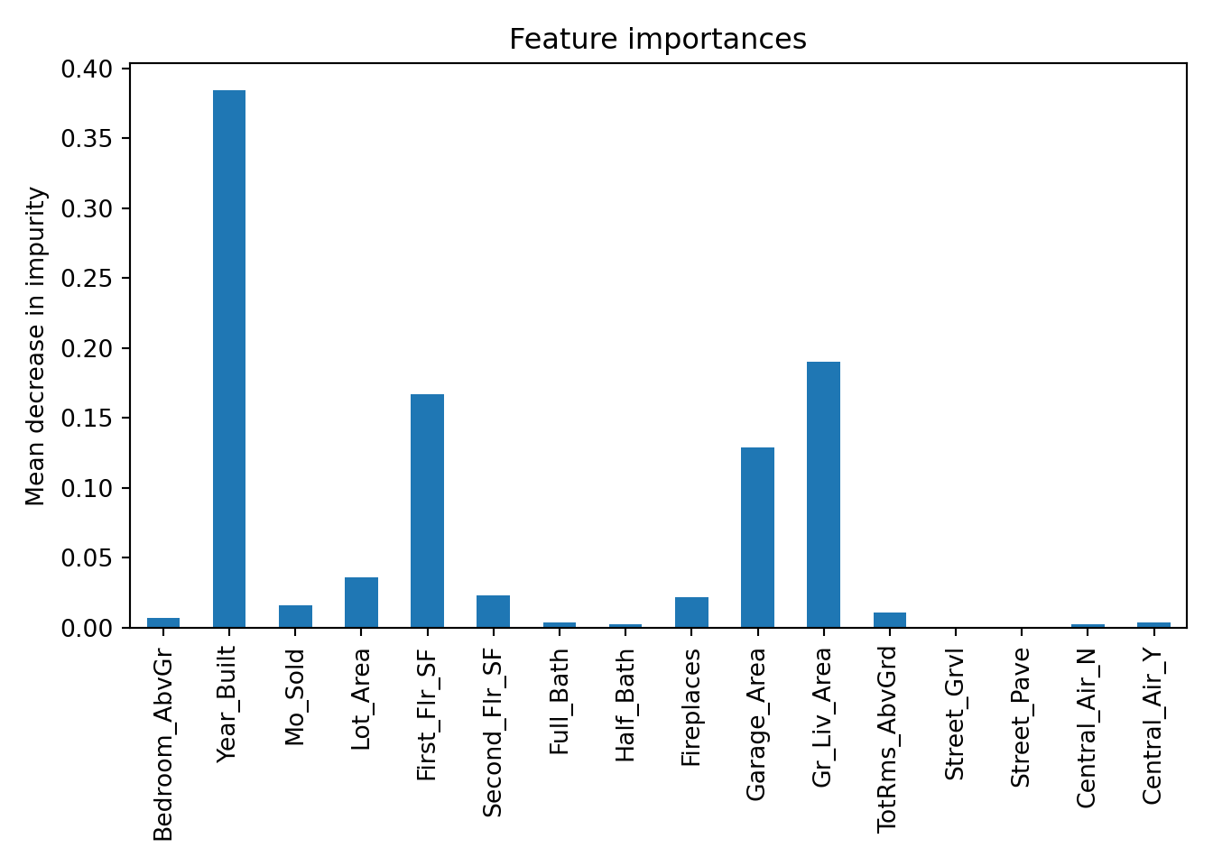
The plot above shows the average decrease in purity in the nodes of the tree - essentially measuring how much each variable improves the purity of the model when it is added. Here, Year_Built is the variable with the most importance.
There are a few things we can tune with a random forest. One is the number of trees used to build the model. Another thing to tune is the number of variables considered for each split - called mtry. By default, \(mtry = \sqrt{p}\), with \(p\) being the number of total variables. We can use cross-validation to tune these values.
Let’s see how to do this in each of our softwares!
In R we can use the tuneRF function to use the out-of-bag samples to tune the mtry variable. These out-of-bag samples serve as cross-validations for each of the trees in the random forest. The values of mtry will be evaluated by the out-of-bag error. The smaller the error, the better.
set.seed(12345)
tuneRF(x = training.df[,-1], y = training.df[,1],
       plot = TRUE, ntreeTry = 500, stepFactor = 0.5)
mtry = 4 OOB error = 877257819
Searching left ...
mtry = 8 OOB error = 886420675
-0.01044488 0.05
Searching right ...
mtry = 2 OOB error = 966299090
-0.1014995 0.05 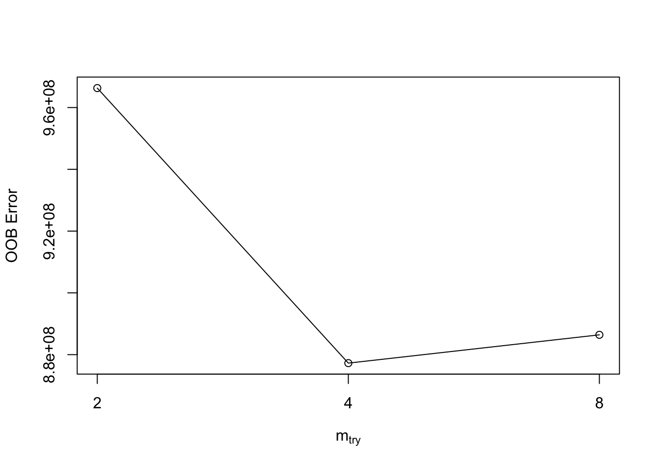
  mtry  OOBError
2    2 966299090
4    4 877257819
8    8 886420675
Based on the output above the value of \(mtry = 4\) is the optimal value. We can then build a model with the 250 trees and \(mtry = 4\) value that was optimized from above.
set.seed(12345)
rf.ames <- randomForest(Sale_Price ~ ., data = training.df, ntree = 250, mtry = 4, importance = TRUE)

varImpPlot(rf.ames,
           sort = TRUE,
           n.var = 14,
           main = "Order of Variables")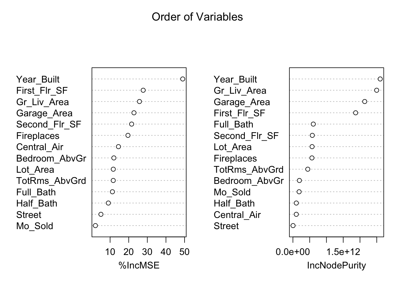
importance(rf.ames, type = 1) %IncMSE
Bedroom_AbvGr 12.021934
Year_Built 49.013449
Mo_Sold 2.105040
Lot_Area 11.714265
Street 5.072419
Central_Air 14.485207
First_Flr_SF 27.776232
Second_Flr_SF 21.568185
Full_Bath 11.247856
Half_Bath 9.059787
Fireplaces 19.593721
Garage_Area 22.819303
Gr_Liv_Area 25.768069
TotRms_AbvGrd 11.695212In Python we can use the GridSearchCV function from the sklearn.model_selection package. In this function we need to define a grid to search across for the parameters to tune. There are 3 parameters to tune in the RandomForestRegressor function - bootstrap which we will leave at True, max_features which is mtry, and n_estimators which is the number of trees.
from sklearn.model_selection import GridSearchCV

param_grid = {
    'bootstrap': [True],
    'max_features': [3, 4, 5, 6, 7],
    'n_estimators': [100, 200, 300, 400, 500, 600, 700, 800]
}

rf = RandomForestRegressor(random_state = 12345)

grid_search = GridSearchCV(estimator = rf, param_grid = param_grid, cv = 10)

grid_search.fit(X_train, y_train)
GridSearchCV(cv=10, estimator=RandomForestRegressor(random_state=12345),
param_grid={'bootstrap': [True], 'max_features': [3, 4, 5, 6, 7],
'n_estimators': [100, 200, 300, 400, 500, 600, 700,
800]})In a Jupyter environment, please rerun this cell to show the HTML representation or trust the notebook. GridSearchCV(cv=10, estimator=RandomForestRegressor(random_state=12345),
param_grid={'bootstrap': [True], 'max_features': [3, 4, 5, 6, 7],
'n_estimators': [100, 200, 300, 400, 500, 600, 700,
800]})RandomForestRegressor(random_state=12345)
RandomForestRegressor(random_state=12345)
grid_search.best_params_{'bootstrap': True, 'max_features': 7, 'n_estimators': 500}Based on the values above, the optimal values for \(mtry\) is 7 and the number of trees is 500.
Another thing to tune would be which variables to include in the random forest. By default, random forests use all the variables since they are averaged across all the trees used to build the model. There are a couple of ways to perform variable selection for random forests:
Many permutations of including/excluding variables
Compare variables to random variable
The first approach is rather straight forward but time consuming because you have to try and build models over and over again taking a variable out each time. The second approach is much easier to try. In that second approach we will create a completely random variable and put it in the model. We will then look at the variable importance of all the variables. The variables that are below the random variable should be considered for removal.
Let’s see this in each of our softwares!
To create a random variable in R we will just use the rnorm function with a mean of 0, standard deviation of 1 (both defaults) and a count of 2051 - the number of observations in our training data.
From there we build the random forest as we previously have.
training.df$random <- rnorm(2051)

set.seed(12345)
rf.ames <- randomForest(Sale_Price ~ ., data = training.df, ntree = 500, mtry = 4, importance = TRUE)

varImpPlot(rf.ames,
           sort = TRUE,
           n.var = 15,
           main = "Look for Variables Below Random Variable")
Based on the plot on the left above, there is no variable below the random variable. However, from the plot on the right, there are 5 variables that could be considered for removal.
To create a random variable in Python we will first create a new data.frame called X_train_r. We will then add a variable called random with the random.normal function from numpy.
import numpy as np

X_train_r = X_train

X_train_r['random'] = np.random.normal(0, 1, 2051)
We then build a random forest model in the same way we did previously and check the variable importance.
rf_ames = RandomForestRegressor(n_estimators = 500,
                                max_features = 7,
                                  random_state = 12345,
                                  oob_score = True)

rf_ames.fit(X_train_r, y_train)
RandomForestRegressor(max_features=7, n_estimators=500, oob_score=True,
random_state=12345)In a Jupyter environment, please rerun this cell to show the HTML representation or trust the notebook. RandomForestRegressor(max_features=7, n_estimators=500, oob_score=True,
random_state=12345)forest_importances = pd.Series(rf_ames.feature_importances_, index = rf_ames.feature_names_in_)
fig, ax = plt.subplots()
forest_importances.plot.bar(ax = ax)
ax.set_title("Feature importances")
ax.set_ylabel("Mean decrease in impurity")
fig.tight_layout()
plt.show()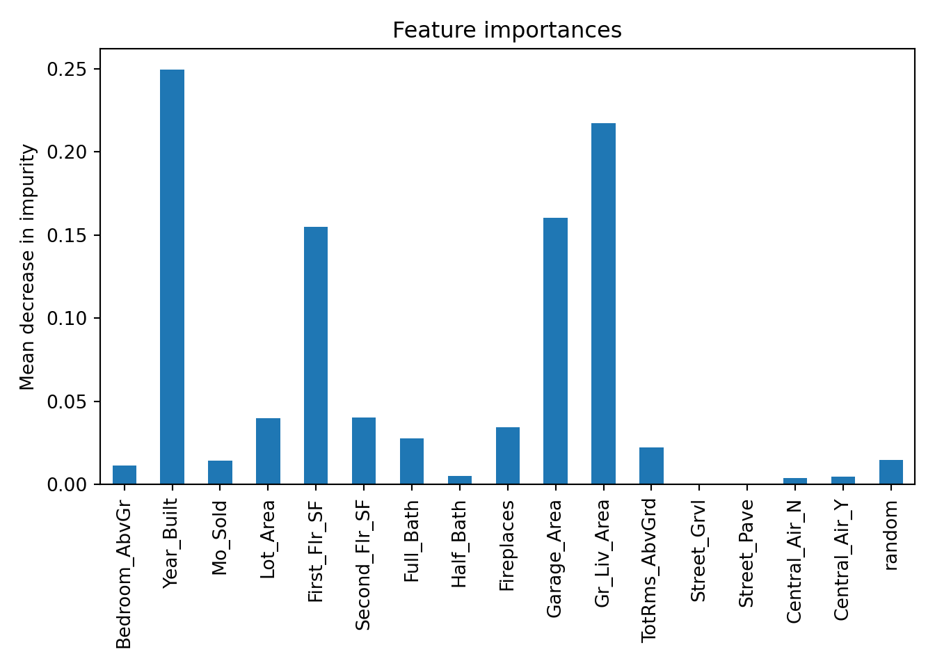
Based on the plot above there are 6 variables that fall below the variable importance of the random variable that could be considered for removal from the model.
Most machine learning models are not interpretable in the classical sense - as one predictor variable increases, the target variable tends to ___. This is because the relationships are not linear. The relationships are more complicated than a linear relationship, so the interpretations are as well. Similar to GAM’s we can get a general idea of an overall pattern for a predictor variable compared to a target variable - partial dependence plots.
These plots will be covered in much more detail in the final section of this code deck under Model Agnostic Interpretability. However, let’s see this in action in R from the options in the randomForest and pdp packages.
partialPlot(rf.ames, training.df, Garage_Area)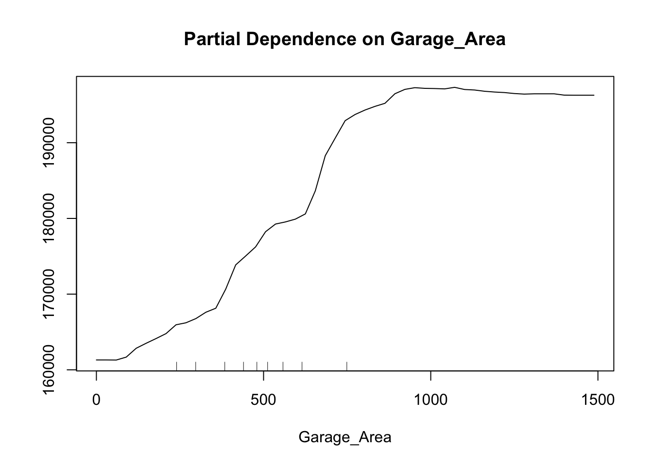
This nonlinear and complex relationship between Garage_Area and Sale_Price is similar to the plot we saw earlier with the GAMs. This shouldn’t be too surprising. Both sets of algorithms are trying to relate these two variables together, just in different ways.
In summary, random forest models are good models to use for prediction, but explanation becomes more difficult and complex. Some of the advantages of using random forests:
Computationally fast (handles thousands of variables)
Trees trained simultaneously
Accurate classification model
Variable importance available
Missing data is OK
There are some disadvantages though:
“Interpretability” is a little different than the classical sense
There are parameters that need to be tuned to make the model the best
Boosting is similar to bagging in the sense that we will draw a sample of observations from a data set with replacement. However, unlike bagging, observations are not sampled randomly. Boosting assigns weights to each training observation and uses the weight as a sampling distribution. Observations with higher weights are more likely to be drawn in the next sample. These weights are changed adaptively in each round. The weights for observations that are harder to classify are higher for the next sample - trying to increase chance of them being selected. We want these missed observations to have a higher chance of being in the next model to improve the chances of predicting those observations correctly the next time. An example of the difference in weights for a boosted sample as compared to a bagging sample is the following:
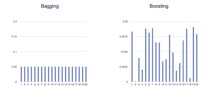
With bagging we are only trying to create variability in the models by using training data set variation. The ensemble model is built simultaneously. However, in boosting, observations with higher sampling probability were harder to predict accurately. We want to improve the predictions from the model sequentially.
Let’s use the same example we used in bagging. The following 10 observations have the values of X and Y shown in the following table:
We will build a decision stump (a decision tree with only one split). From building a decision stump, the best accuracy is obtained by making the split at either 3.5 or 7.5. Either of these splits would lead to an accuracy of predicting Y at 70%. For example, let’s use the split at 3.5. That would mean we think everything above 3.5 is a 0 and everything below 3.5 is a 1. We would get observations 1, 2, and 3 all correct. However, since everything above 3.5 is considered a 0, we would only get observations 4, 5, 6, and 7 correct on that half - missing observations 8, 9, and 10.
To try and make this prediction better we will do the following:
Take 3 bootstrap samples
Build a decision stump for each
At each step we will adjust the weights based on the previous step’s errors
The following is the first 3 bootstrap samples with their optimal splits. Remember, these bootstrap samples will not contain all of the observations in the original data set.
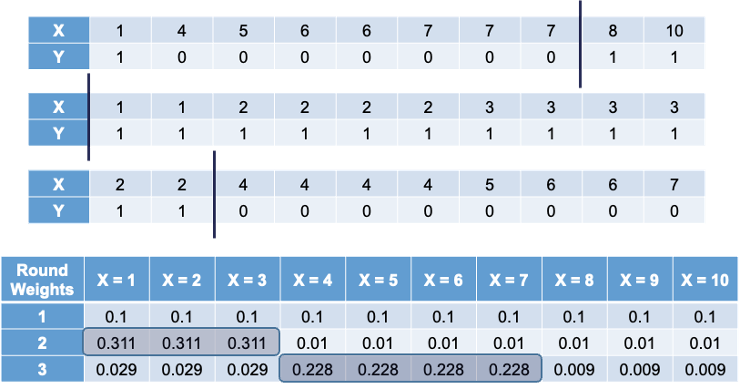
The first sample has the same weight for each observation. In that bootstrap sample the best split occurs at 7.5. However, when predicting the original observations, we would incorrectly predict observations 1, 2, and 3. Therefore, in the second sample we will overweight observations 1, 2, and 3 to help us predict those observations better (correct for the previous mistakes). In the second bootstrap sample we have observations 1, 2, and 3 over-represented by design. However, this leads to incorrect predictions in observations 4 through 7. This will lead to us over-weighting those observations as seen in the third row of the weights table. Observations 8, 9, and 10 have always been correctly predicted so their weight is the smallest, while the other observations have higher weights.
The original boosted sample ensemble was called AdaBoost. Unlike bagging, boosted ensembles usually weight the votes of each classifier by a function of their accuracy. If the classifier gets the higher weighted observations wrong, it has a higher error rate. More accurate classifiers get a higher weight in the prediction. In simple terms, more accurate guesses are more important. We will not detail this algorithm here as there are more common advancements that have come since.
Some more recent algorithms are moving away from the direct boosting approach applied to bootstrap samples. However, the main idea of these algorithms is still rooted in the notion of finding where you made mistakes and trying to improve on those mistakes.
One of the original algorithms to go with this approach is the gradient boosted machine (GBM). The idea behind the GBM is to build a simple model to predict the target (much like a decision tree or even decision stump):
\[ y = f_1(x) + \varepsilon_1 \]
That simple model has an error of \(\varepsilon_1\). The next step is to try to predict that error with another simple model:
\[ \varepsilon_1 = f_2(x) + \varepsilon_2 \]
This model has an error of \(\varepsilon_2\). We can continue to add model after model, each one predicting the error (residuals) from the previous round:
\[ y = f_1(x) + f_2(x) + \cdots + f_k(x) + \varepsilon_k \]
We will continue this process until there is a really small error which will lead to over-fitting. To protect against over-fitting, we will build in gradient boosting regularization through parameters to tune. One of those parameters to tune is \(\eta\), which is the weight applied to the error models:
\[ y = f_1(x) + \eta \times f_2(x) + \eta \times f_3(x) + \cdots + \eta \times f_k(x) + \varepsilon_k \]
Smaller values of \(\eta\) lead to less over-fitting. Other things to tune include the number of trees to use in the prediction (more trees typically lead to more over-fitting), and other parameters added over the years - \(\lambda\), \(\gamma\), \(L_2\), etc.
Gradient boosting as defined above yields an additive ensemble model. There is no voting or averaging of individual models as the models are built sequentially, not simultaneously. The predictions from these models are added together to get the final prediction. One of the big keys to gradient boosting is using weak learners. Weak learners are simple models. Shallow decision / regression trees are the best. Each of these models would make poor predictions on their own, but the additive fashion of the ensemble provides really good predictions.
These models are optimized to some form of a loss function. For example, linear regression looks at minimizing the sum of squared errors - its loss function. The sum of squared errors from many predictions would aggregate into a single number - the loss of the whole model. Gradient boosting is much the same, but not limited to sum of squared errors for the loss function.
How does the gradient boosting model find this optimal loss function value? It uses gradient descent. Gradient descent is a method that iteratively updates parameters in order to minimize a loss function (the sum of squared errors for example) by moving in the direction of the steepest descent as seen in the figure below:
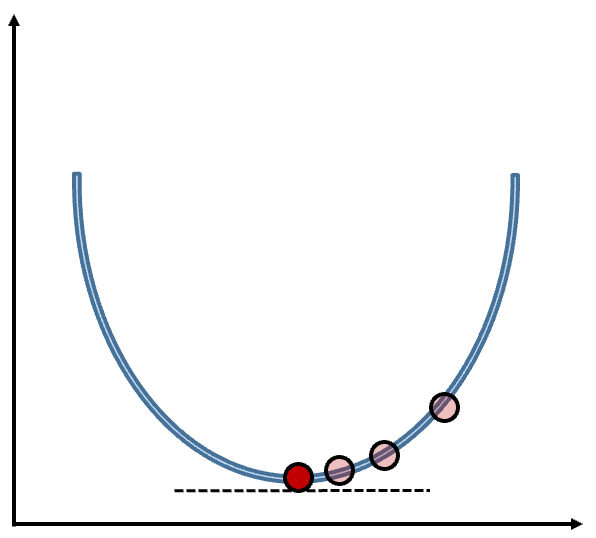
This function minimizes the loss function by taking iteratively smaller steps until it finds the minimum. The step size is updated at each step to help with the minimization. The step size is updated with the learning rate. Without the learning rate, we might take steps too big and miss the minimum or too small and take a long time to optimize.
Not all functions are convex as some have local minimums or plateaus that make finding the global minimum difficult. Stochastic gradient descent attempts to solve this problem by randomly sampling a fraction of the training observations for each tree in the ensemble - not all trees contain the all of the observations. This makes the algorithm faster and more reliable, but may not always find the true overall minimum.
Grid search for these algorithms are very time consuming because of the time it takes ot build these models since they are built sequentially. To speed up this process, we typically set the tuning parameters to default and optimize the number of trees in the GBM. We then fix the tree count and start to tune other parameters. Then we go back and iteratively tune back and forth until we find an optimal solution.
There are many different adaptations to the gradient boosting approach:
XGBoost
LightGBM
CatBoost
etc.
Extreme gradient boosting (XGBoost) is one of the most popular versions of these algorithms. XGBoost has some great advantages over the traditional GBM:
Let’s see how to build this in each of our softwares!
To build this model in R we first need to get the data in the right format. We need separate data matrices for our predictors and our target variable. First, we use the model.matrix function will create any categorical dummy variables needed. We also isolate the target variable into its own vector.
train_x <- model.matrix(Sale_Price ~ ., data = training)[, -1]
train_y <- training$Sale_Price
Next, we will use the xgboost package and the xgboost function. First we will set the seed to make the results repeatable. Then, with the xgboost function we give the predictor variable model.matrix in the data = option. The label = option is where we specify the target variable. The subsample = 0.5 option is specifying that we will use stochastic gradient descent and only use a random 50% of the training data for each tree. The number of trees (nrounds) is set to 50.
library(xgboost)

set.seed(12345)
xgb.ames <- xgboost(data = train_x, label = train_y, subsample = 0.5, nrounds = 50)
[1] train-rmse:142608.463852
[2] train-rmse:103674.675174
[3] train-rmse:76943.862703
[4] train-rmse:58578.815950
[5] train-rmse:45371.238589
[6] train-rmse:36946.279173
[7] train-rmse:31558.903651
[8] train-rmse:28006.968483
[9] train-rmse:25683.987255
[10] train-rmse:24168.869119
[11] train-rmse:22783.641756
[12] train-rmse:22078.056141
[13] train-rmse:21693.474938
[14] train-rmse:21248.689369
[15] train-rmse:20759.314997
[16] train-rmse:20274.597822
[17] train-rmse:19901.853233
[18] train-rmse:19499.755714
[19] train-rmse:19227.633174
[20] train-rmse:18925.576092
[21] train-rmse:18659.121774
[22] train-rmse:18149.635690
[23] train-rmse:17791.386187
[24] train-rmse:17694.197535
[25] train-rmse:17460.768708
[26] train-rmse:17141.923149
[27] train-rmse:16934.683648
[28] train-rmse:16686.018910
[29] train-rmse:16556.936678
[30] train-rmse:16299.041062
[31] train-rmse:16143.484613
[32] train-rmse:15729.010037
[33] train-rmse:15467.075227
[34] train-rmse:15289.998639
[35] train-rmse:14963.258359
[36] train-rmse:14847.081551
[37] train-rmse:14673.496223
[38] train-rmse:14489.353996
[39] train-rmse:14296.691986
[40] train-rmse:14084.853151
[41] train-rmse:13769.683684
[42] train-rmse:13621.880172
[43] train-rmse:13398.597729
[44] train-rmse:13111.253799
[45] train-rmse:13014.121445
[46] train-rmse:12770.213707
[47] train-rmse:12613.208916
[48] train-rmse:12468.561979
[49] train-rmse:12255.996904
[50] train-rmse:12067.771479 That will build a model for us, but we need to start tuning the model. For tuning the model, we will use the function xgb.cv. This function will tune the number of trees (nrounds) variable. The rest of the inputs are the same as the xgboost function above. The only additional option is the nfold = option that sets the number of folds in the cross-validation.
xgbcv.ames <- xgb.cv(data = train_x, label = train_y, subsample = 0.5, nrounds = 50, nfold = 10)[1] train-rmse:142038.124133+680.486692 test-rmse:142434.395067+5731.140470
[2] train-rmse:103637.646415+613.092331 test-rmse:104728.052962+5067.596533
[3] train-rmse:76760.598269+459.805754 test-rmse:78965.225482+5608.382458
[4] train-rmse:58494.873543+454.382338 test-rmse:61704.391943+5745.425491
[5] train-rmse:45759.873463+649.534435 test-rmse:50174.953424+5820.072176
[6] train-rmse:37326.883619+615.935175 test-rmse:42669.301738+5558.347487
[7] train-rmse:31771.994582+676.524025 test-rmse:38081.238598+5573.236746
[8] train-rmse:27931.915319+622.837890 test-rmse:35433.022275+5575.618933
[9] train-rmse:25499.729536+630.488841 test-rmse:33579.170630+5153.759721
[10] train-rmse:23988.967462+591.150400 test-rmse:32837.527415+4634.556489
[11] train-rmse:22822.568637+570.688573 test-rmse:32443.570364+4592.312596
[12] train-rmse:21943.245851+511.978457 test-rmse:31871.176282+4270.133588
[13] train-rmse:21364.156799+514.270645 test-rmse:31665.567123+4133.337655
[14] train-rmse:20830.284278+520.305955 test-rmse:31424.545392+4168.372763
[15] train-rmse:20409.575120+528.717464 test-rmse:31471.128497+4000.168663
[16] train-rmse:20059.098516+561.641584 test-rmse:31366.356847+3875.603567
[17] train-rmse:19619.019488+540.497007 test-rmse:31189.196904+3913.209989
[18] train-rmse:19322.152568+525.975024 test-rmse:31304.141382+3944.118954
[19] train-rmse:19020.194006+571.238924 test-rmse:31418.142855+3952.239816
[20] train-rmse:18753.190204+579.649353 test-rmse:31308.422462+3860.782837
[21] train-rmse:18448.374597+522.920719 test-rmse:31254.113018+4008.558610
[22] train-rmse:18137.292830+495.801082 test-rmse:31292.874087+3867.134132
[23] train-rmse:17916.729747+467.278588 test-rmse:31287.967577+3881.147656
[24] train-rmse:17602.418932+465.324487 test-rmse:31065.138000+3663.766297
[25] train-rmse:17332.210614+516.379948 test-rmse:31103.798735+3625.928379
[26] train-rmse:17046.302509+483.072938 test-rmse:31200.873021+3611.565480
[27] train-rmse:16771.223416+468.129136 test-rmse:31176.902969+3717.704813
[28] train-rmse:16517.049640+425.809352 test-rmse:31297.816200+3691.242575
[29] train-rmse:16252.489279+457.047986 test-rmse:31305.349499+3684.384852
[30] train-rmse:16034.356296+469.903404 test-rmse:31347.551234+3793.695249
[31] train-rmse:15783.829117+438.470601 test-rmse:31420.018264+3879.185302
[32] train-rmse:15558.806541+448.600706 test-rmse:31495.762351+3886.447496
[33] train-rmse:15342.650230+410.478632 test-rmse:31561.744649+3853.841647
[34] train-rmse:15150.580911+446.969418 test-rmse:31578.980392+3849.616631
[35] train-rmse:14884.277072+480.560196 test-rmse:31579.307217+3845.204612
[36] train-rmse:14672.387053+484.909533 test-rmse:31543.387284+3806.607373
[37] train-rmse:14456.533952+447.632857 test-rmse:31549.985429+3882.599118
[38] train-rmse:14246.502944+464.202936 test-rmse:31579.370253+3892.624114
[39] train-rmse:14044.030664+461.818885 test-rmse:31621.703722+3796.825057
[40] train-rmse:13840.366069+483.067658 test-rmse:31602.805317+3829.811513
[41] train-rmse:13671.402239+517.465905 test-rmse:31582.314907+3838.929718
[42] train-rmse:13483.542367+524.601114 test-rmse:31598.410650+3855.253641
[43] train-rmse:13301.392103+530.910573 test-rmse:31629.765353+3898.496750
[44] train-rmse:13102.955975+534.254162 test-rmse:31636.679048+3874.856098
[45] train-rmse:12922.787101+539.528266 test-rmse:31596.089510+3930.760861
[46] train-rmse:12721.871308+521.349722 test-rmse:31646.292901+3902.644066
[47] train-rmse:12547.384795+499.943536 test-rmse:31698.393853+3896.584705
[48] train-rmse:12386.962779+484.783823 test-rmse:31661.231013+3932.004582
[49] train-rmse:12213.191861+504.465304 test-rmse:31693.565032+3976.567381
[50] train-rmse:12044.942280+495.047422 test-rmse:31658.189792+3976.543524 From the output above we can see two columns. The left hand column is the RMSE from all the models built on the training data. As the number of trees increases, the RMSE is getting better and better which isn’t surprising as the errors from one will inform the next tree. However, the right hand column is the RMSE on the validation (test by name above) data, which is not guaranteed to improve as the number of trees increases. This validation evaluation will help us evaluate the “best” number of trees. We can see that the validation RMSE is minimized at 24 trees.
Now that we know that 24 trees in the model is the optimized number (under the default tuning of the other parameters) we can move to tuning the other parameters. We will again use the train function from caret. We will use many different parameters in the tuning. Inside the tuneGrid option we will fix the nrounds to 24 (as determined above), the gamma value to 0, and the colsample_bytree and min_child_weight to be 1. We will change the eta value to be one of 5 values, max_depth to be one of 10 values, and subsample to be one of 4 values. Inside the train function we will still use the 10 fold cross-validation as before. For the method option we have the xgbTree value. The plot function will provide a plot comparing all of these tuning parameter values.
library(caret)

tune_grid <- expand.grid(
  nrounds = 24,
  eta = c(0.1, 0.15, 0.2, 0.25, 0.3),
  max_depth = c(1:10),
  gamma = c(0),
  colsample_bytree = 1,
  min_child_weight = 1,
  subsample = c(0.25, 0.5, 0.75, 1)
)

set.seed(12345)
xgb.ames.caret <- train(x = train_x, y = train_y,
      method = "xgbTree",
      tuneGrid = tune_grid,
      trControl = trainControl(method = 'cv', # Using 10-fold cross-validation
                               number = 10))

plot(xgb.ames.caret)
xgb.ames.caret$bestTune nrounds max_depth eta gamma colsample_bytree min_child_weight subsample
144 24 6 0.25 0 1 1 1The lowest RMSE on cross-validation occurs where a maximum tree depth is 6, the subsample is 100% (not stochastic; has the whole sample), and \(\eta\) is 0.25.
To truly optimize the XGBoost model, we would take these values and try to optimize the nrounds as we did before under these new values for the other parameters. We would then redo the tuning of these other parameters under the new number of trees and shrink the grid to get more exact values of each tuning parameter. This process is rather time consuming so be prepared.
To build this model in Python We will use the XGBRegressor function from the xgboost package. Similar to other Python functions we have used, we need the training predictor variables in one object and the target variable in another. These will be passed to the .fit portion of the code below. The options for the XGBoost model are n_estimators to define how many trees we need. The subsample = 0.5 option is specifying that we will use stochastic gradient descent and only use a random 50% of the training data for each tree. The number of trees (n_estimators) is set to 50. We are also setting a seed to make the results repeatable.
from xgboost import XGBRegressor

xgb_ames = XGBRegressor(n_estimators = 50,
                        subsample = 0.5,
                        random_state = 12345)

xgb_ames.fit(X_train, y_train)
XGBRegressor(base_score=None, booster=None, callbacks=None,
colsample_bylevel=None, colsample_bynode=None,
colsample_bytree=None, device=None, early_stopping_rounds=None,
enable_categorical=False, eval_metric=None, feature_types=None,
gamma=None, grow_policy=None, importance_type=None,
interaction_constraints=None, learning_rate=None, max_bin=None,
max_cat_threshold=None, max_cat_to_onehot=None,
max_delta_step=None, max_depth=None, max_leaves=None,
min_child_weight=None, missing=nan, monotone_constraints=None,
multi_strategy=None, n_estimators=50, n_jobs=None,
num_parallel_tree=None, random_state=12345, ...)In a Jupyter environment, please rerun this cell to show the HTML representation or trust the notebook. XGBRegressor(base_score=None, booster=None, callbacks=None,
colsample_bylevel=None, colsample_bynode=None,
colsample_bytree=None, device=None, early_stopping_rounds=None,
enable_categorical=False, eval_metric=None, feature_types=None,
gamma=None, grow_policy=None, importance_type=None,
interaction_constraints=None, learning_rate=None, max_bin=None,
max_cat_threshold=None, max_cat_to_onehot=None,
max_delta_step=None, max_depth=None, max_leaves=None,
min_child_weight=None, missing=nan, monotone_constraints=None,
multi_strategy=None, n_estimators=50, n_jobs=None,
num_parallel_tree=None, random_state=12345, ...)That will build a model for us, but we need to start tuning the model. For tuning the model, we will use the function GridSearchCV that we used before with random forests. In this function we need to define a grid to search across for the parameters to tune. There are many parameters we can tune in the XGBRegressor function. We will look at tuning the number of trees in the XGBoost model (n_estimators) with values of 5 through 50 by 5, eta to be one of 5 values, max_depth to be one of 10 values, and subsample to be one of 4 values. We will continue to use a 10 fold cross-validation to evaluate these tuning parameters.
param_grid = {
    'n_estimators': [5, 10, 15, 20, 25, 30, 35, 40, 45, 50],
    'eta': [0.1, 0.15, 0.2, 0.25, 0.3],
    'max_depth': [1, 2, 3, 4, 5, 6, 7, 8, 9, 10],
    'subsample': [0.25, 0.5, 0.75, 1]
}

xgb = XGBRegressor()

grid_search = GridSearchCV(estimator = xgb, param_grid = param_grid, cv = 10)

grid_search.fit(X_train, y_train)
GridSearchCV(cv=10,
estimator=XGBRegressor(base_score=None, booster=None,
callbacks=None, colsample_bylevel=None,
colsample_bynode=None,
colsample_bytree=None, device=None,
early_stopping_rounds=None,
enable_categorical=False, eval_metric=None,
feature_types=None, gamma=None,
grow_policy=None, importance_type=None,
interaction_constraints=None,
learning_rate=None,...
max_cat_to_onehot=None, max_delta_step=None,
max_depth=None, max_leaves=None,
min_child_weight=None, missing=nan,
monotone_constraints=None,
multi_strategy=None, n_estimators=None,
n_jobs=None, num_parallel_tree=None,
random_state=None, ...),
param_grid={'eta': [0.1, 0.15, 0.2, 0.25, 0.3],
'max_depth': [1, 2, 3, 4, 5, 6, 7, 8, 9, 10],
'n_estimators': [5, 10, 15, 20, 25, 30, 35, 40, 45,
50],
'subsample': [0.25, 0.5, 0.75, 1]})In a Jupyter environment, please rerun this cell to show the HTML representation or trust the notebook. GridSearchCV(cv=10,
estimator=XGBRegressor(base_score=None, booster=None,
callbacks=None, colsample_bylevel=None,
colsample_bynode=None,
colsample_bytree=None, device=None,
early_stopping_rounds=None,
enable_categorical=False, eval_metric=None,
feature_types=None, gamma=None,
grow_policy=None, importance_type=None,
interaction_constraints=None,
learning_rate=None,...
max_cat_to_onehot=None, max_delta_step=None,
max_depth=None, max_leaves=None,
min_child_weight=None, missing=nan,
monotone_constraints=None,
multi_strategy=None, n_estimators=None,
n_jobs=None, num_parallel_tree=None,
random_state=None, ...),
param_grid={'eta': [0.1, 0.15, 0.2, 0.25, 0.3],
'max_depth': [1, 2, 3, 4, 5, 6, 7, 8, 9, 10],
'n_estimators': [5, 10, 15, 20, 25, 30, 35, 40, 45,
50],
'subsample': [0.25, 0.5, 0.75, 1]})XGBRegressor(base_score=None, booster=None, callbacks=None,
colsample_bylevel=None, colsample_bynode=None,
colsample_bytree=None, device=None, early_stopping_rounds=None,
enable_categorical=False, eval_metric=None, feature_types=None,
gamma=None, grow_policy=None, importance_type=None,
interaction_constraints=None, learning_rate=None, max_bin=None,
max_cat_threshold=None, max_cat_to_onehot=None,
max_delta_step=None, max_depth=None, max_leaves=None,
min_child_weight=None, missing=nan, monotone_constraints=None,
multi_strategy=None, n_estimators=None, n_jobs=None,
num_parallel_tree=None, random_state=None, ...)XGBRegressor(base_score=None, booster=None, callbacks=None,
colsample_bylevel=None, colsample_bynode=None,
colsample_bytree=None, device=None, early_stopping_rounds=None,
enable_categorical=False, eval_metric=None, feature_types=None,
gamma=None, grow_policy=None, importance_type=None,
interaction_constraints=None, learning_rate=None, max_bin=None,
max_cat_threshold=None, max_cat_to_onehot=None,
max_delta_step=None, max_depth=None, max_leaves=None,
min_child_weight=None, missing=nan, monotone_constraints=None,
multi_strategy=None, n_estimators=None, n_jobs=None,
num_parallel_tree=None, random_state=None, ...)grid_search.best_params_{'eta': 0.15, 'max_depth': 5, 'n_estimators': 50, 'subsample': 0.75}The lowest RMSE on cross-validation occurs where a maximum tree depth is 5, the subsample is 75% (stochastic; has 75% sample), \(\eta\) is 0.15, and uses 50 trees in the model.
To truly optimize the XGBoost model, we would take these values and try to shrink the grid to get more exact values of each tuning parameter. This process is rather time consuming so be prepared.
XGBoost provides three built-in measures of variable importance:
Let’s see this in each of our softwares!
To look at variable importance of an XGBoost model in R we just use the xbg.importance function. First we build an XGBoost model with the parameters tuned to the optimal values from the previous section. Then we put this model into the xgb.importance function. If we wanted to visualize these we could use the xgb.ggplot.importance function on the variable importance object.
xgb.ames <- xgboost(data = train_x, label = train_y, subsample = 1, nrounds = 24, eta = 0.25, max_depth = 5)[1] train-rmse:150443.019681
[2] train-rmse:115268.490408
[3] train-rmse:89057.171941
[4] train-rmse:69562.543066
[5] train-rmse:55214.634015
[6] train-rmse:44735.716089
[7] train-rmse:37067.488868
[8] train-rmse:31645.067008
[9] train-rmse:27828.776299
[10] train-rmse:25306.722264
[11] train-rmse:23565.984940
[12] train-rmse:22392.109885
[13] train-rmse:21511.520180
[14] train-rmse:20955.373384
[15] train-rmse:20432.494270
[16] train-rmse:20020.723800
[17] train-rmse:19687.918549
[18] train-rmse:19469.456955
[19] train-rmse:19024.269445
[20] train-rmse:18796.187111
[21] train-rmse:18659.664360
[22] train-rmse:18561.140970
[23] train-rmse:18362.762981
[24] train-rmse:18284.120276 xgb.importance(feature_names = colnames(train_x), model = xgb.ames) Feature Gain Cover Frequency
<char> <num> <num> <num>
1: Year_Built 0.4090163675 0.171166757 0.165794066
2: Gr_Liv_Area 0.2166471415 0.198657323 0.136125654
3: Garage_Area 0.1497264247 0.089070744 0.111692845
4: First_Flr_SF 0.1309835527 0.150797929 0.143106457
5: Fireplaces 0.0390155028 0.046181049 0.033158813
6: Lot_Area 0.0194787474 0.167614054 0.155322862
7: Second_Flr_SF 0.0112451543 0.027167965 0.040139616
8: Mo_Sold 0.0059546058 0.013181751 0.071553229
9: Bedroom_AbvGr 0.0055976867 0.053764231 0.066317627
10: Central_AirY 0.0046784371 0.017898270 0.010471204
11: Half_Bath 0.0037108953 0.022749547 0.027923211
12: TotRms_AbvGrd 0.0029567060 0.005998759 0.024432810
13: Full_Bath 0.0008079959 0.024207380 0.010471204
14: StreetPave 0.0001807826 0.011544241 0.003490401xgb.ggplot.importance(xgb.importance(feature_names = colnames(train_x), model = xgb.ames))
From the output above we see the variables in the model ranked by gain for variable importance. The plot above is also in terms of gain. The nice part about the plot is that it clusters the variables together that have similar gain. From the above output we have 3 clusters of variables. The first cluster has Year_Built all by itself. The second cluster has Gr_Liv_Area, Garage_Area, and First_Flr_SF. The last cluster has all the remaining variables.
To look at variable importance of an XGBoost model in Python we just use the feature_importances_ element from the XGBRegressor model object. First we build an XGBoost model with the parameters tuned to the optimal values from the previous section. Next, we are plotting the feature_importance_ values against the names of the variables.
xgb_ames = XGBRegressor(n_estimators = 50,
                        subsample = 0.75,
                        eta = 0.15,
                        max_depth = 5,
                        random_state = 12345)

xgb_ames.fit(X_train, y_train)
XGBRegressor(base_score=None, booster=None, callbacks=None,
colsample_bylevel=None, colsample_bynode=None,
colsample_bytree=None, device=None, early_stopping_rounds=None,
enable_categorical=False, eta=0.15, eval_metric=None,
feature_types=None, gamma=None, grow_policy=None,
importance_type=None, interaction_constraints=None,
learning_rate=None, max_bin=None, max_cat_threshold=None,
max_cat_to_onehot=None, max_delta_step=None, max_depth=5,
max_leaves=None, min_child_weight=None, missing=nan,
monotone_constraints=None, multi_strategy=None, n_estimators=50,
n_jobs=None, num_parallel_tree=None, ...)In a Jupyter environment, please rerun this cell to show the HTML representation or trust the notebook. XGBRegressor(base_score=None, booster=None, callbacks=None,
colsample_bylevel=None, colsample_bynode=None,
colsample_bytree=None, device=None, early_stopping_rounds=None,
enable_categorical=False, eta=0.15, eval_metric=None,
feature_types=None, gamma=None, grow_policy=None,
importance_type=None, interaction_constraints=None,
learning_rate=None, max_bin=None, max_cat_threshold=None,
max_cat_to_onehot=None, max_delta_step=None, max_depth=5,
max_leaves=None, min_child_weight=None, missing=nan,
monotone_constraints=None, multi_strategy=None, n_estimators=50,
n_jobs=None, num_parallel_tree=None, ...)forest_importances = pd.Series(xgb_ames.feature_importances_, index = xgb_ames.feature_names_in_)
fig, ax = plt.subplots()
forest_importances.plot.bar(ax = ax)
ax.set_title("Feature importances")
ax.set_ylabel("Mean decrease in impurity")
fig.tight_layout()
plt.show()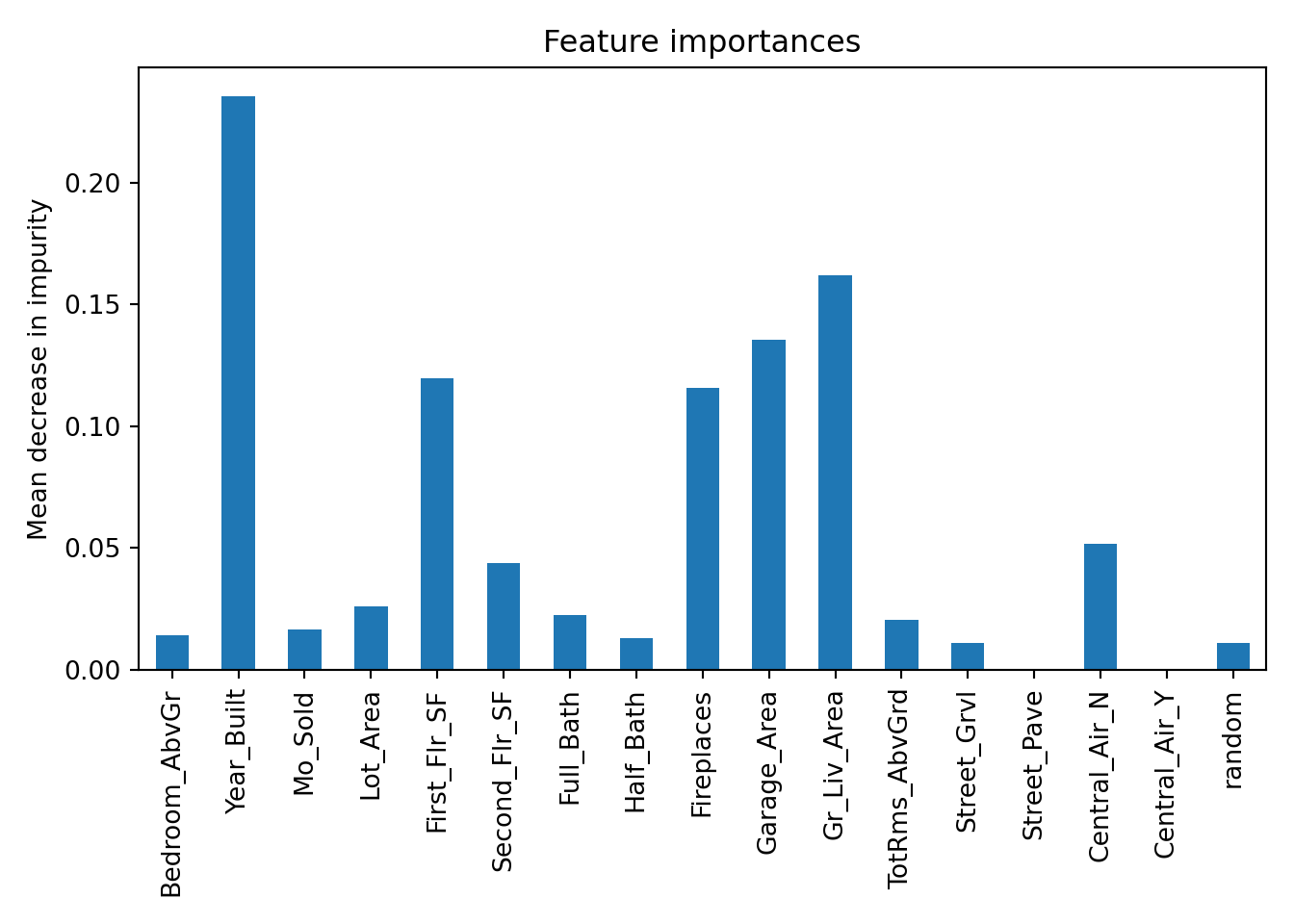
The plot above has the variables ranked by gain. We can see that Year_Built is the best variable by far. This is followed by First_Flr_SF, Garage_Area, and Gr_Liv_Area.
Another way to plot the importance is with the plot_importance function from the xgboost package.
import xgboost

xgboost.plot_importance(xgb_ames, importance_type = 'cover')

plt.show()
Another thing to tune would be which variables to include in the XGBoost model. By default, XGBoost use all the variables since they are aggregated across all the trees used to build the model. There are a couple of ways to perform variable selection for XGBoost:
Many permutations of including/excluding variables
Compare variables to random variable
The first approach is rather straight forward but time consuming because you have to try and build models over and over again taking a variable out each time. The second approach is much easier to try. In that second approach we will create a completely random variable and put it in the model. We will then look at the variable importance of all the variables. The variables that are below the random variable should be considered for removal.
Let’s see this in each of our softwares!
To create a random variable in R we will just use the rnorm function with a mean of 0, standard deviation of 1 (both defaults) and a count of 2051 - the number of observations in our training data.
From there we build the XGBoost model as we previously have.
training$random <- rnorm(2051)

train_x <- model.matrix(Sale_Price ~ ., data = training)[, -1]
train_y <- training$Sale_Price

set.seed(12345)
xgb.ames <- xgboost(data = train_x, label = train_y, subsample = 1, nrounds = 24, eta = 0.25, max_depth = 5, objective = "reg:linear")
[12:20:51] WARNING: src/objective/regression_obj.cu:213: reg:linear is now deprecated in favor of reg:squarederror.
[1] train-rmse:150443.019681
[2] train-rmse:115267.504962
[3] train-rmse:89055.111389
[4] train-rmse:69561.730180
[5] train-rmse:55220.286080
[6] train-rmse:44740.341203
[7] train-rmse:36980.683350
[8] train-rmse:31451.655598
[9] train-rmse:27650.915529
[10] train-rmse:24945.269999
[11] train-rmse:23211.562386
[12] train-rmse:22012.817481
[13] train-rmse:21221.348708
[14] train-rmse:20602.110276
[15] train-rmse:20145.482316
[16] train-rmse:19789.451818
[17] train-rmse:19549.927138
[18] train-rmse:19182.487244
[19] train-rmse:19050.917338
[20] train-rmse:18579.468210
[21] train-rmse:18479.830197
[22] train-rmse:18164.219167
[23] train-rmse:18008.414679
[24] train-rmse:17887.039967 xgb.importance(feature_names = colnames(train_x), model = xgb.ames) Feature Gain Cover Frequency
<char> <num> <num> <num>
1: Year_Built 0.4067193102 0.183708803 0.140819964
2: Gr_Liv_Area 0.2179078887 0.192822988 0.121212121
3: Garage_Area 0.1492481940 0.094004320 0.110516934
4: First_Flr_SF 0.1288022095 0.143082897 0.149732620
5: Fireplaces 0.0380211639 0.046918450 0.033868093
6: Lot_Area 0.0187551693 0.146431299 0.128342246
7: Second_Flr_SF 0.0097506682 0.043431213 0.055258467
8: random 0.0069491993 0.008125998 0.069518717
9: Mo_Sold 0.0054516148 0.008260751 0.051693405
10: Bedroom_AbvGr 0.0052478631 0.049740091 0.053475936
11: Central_AirY 0.0046903553 0.018367205 0.012477718
12: TotRms_AbvGrd 0.0037997281 0.015582316 0.030303030
13: Half_Bath 0.0034109167 0.025202844 0.026737968
14: Full_Bath 0.0009226264 0.005692282 0.010695187
15: StreetPave 0.0003230926 0.018628544 0.005347594xgb.ggplot.importance(xgb.importance(feature_names = colnames(train_x), model = xgb.ames))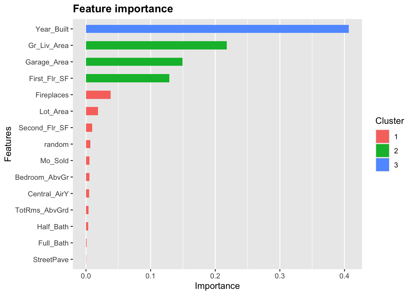
Based on the plot above we can see 7 variables that are below the random variable in terms of gain. These could be considered for removal from the model. However, We can see that there are 3 variables above random, but considered to be similar to random based on the cluster they are in. You could consider to remove these as well. As always though, the main focus is on prediction here and not necessarily on model parsimony.
To create a random variable in Python we will first create a new data.frame called X_train_r. We will then add a variable called random with the random.normal function from numpy. We then build an XGBoost model in the same way we did previously and check the variable importance.
import numpy as np

X_train_r = X_train

X_train_r['random'] = np.random.normal(0, 1, 2051)xgb_ames = XGBRegressor(n_estimators = 50,
subsample = 0.75,
eta = 0.15,
max_depth = 5,
random_state = 12345)
xgb_ames.fit(X_train_r, y_train)XGBRegressor(base_score=None, booster=None, callbacks=None,
colsample_bylevel=None, colsample_bynode=None,
colsample_bytree=None, device=None, early_stopping_rounds=None,
enable_categorical=False, eta=0.15, eval_metric=None,
feature_types=None, gamma=None, grow_policy=None,
importance_type=None, interaction_constraints=None,
learning_rate=None, max_bin=None, max_cat_threshold=None,
max_cat_to_onehot=None, max_delta_step=None, max_depth=5,
max_leaves=None, min_child_weight=None, missing=nan,
monotone_constraints=None, multi_strategy=None, n_estimators=50,
n_jobs=None, num_parallel_tree=None, ...)In a Jupyter environment, please rerun this cell to show the HTML representation or trust the notebook. XGBRegressor(base_score=None, booster=None, callbacks=None,
colsample_bylevel=None, colsample_bynode=None,
colsample_bytree=None, device=None, early_stopping_rounds=None,
enable_categorical=False, eta=0.15, eval_metric=None,
feature_types=None, gamma=None, grow_policy=None,
importance_type=None, interaction_constraints=None,
learning_rate=None, max_bin=None, max_cat_threshold=None,
max_cat_to_onehot=None, max_delta_step=None, max_depth=5,
max_leaves=None, min_child_weight=None, missing=nan,
monotone_constraints=None, multi_strategy=None, n_estimators=50,
n_jobs=None, num_parallel_tree=None, ...)forest_importances = pd.Series(xgb_ames.feature_importances_, index = xgb_ames.feature_names_in_)
fig, ax = plt.subplots()
forest_importances.plot.bar(ax = ax)
ax.set_title("Feature importances")
ax.set_ylabel("Mean decrease in impurity")
fig.tight_layout()
plt.show()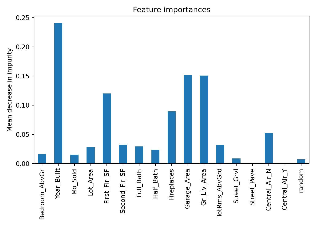
Based on the plot above there are 2 variables that fall below the variable importance of the random variable that could be considered for removal from the model.
Most machine learning models are not interpretable in the classical sense - as one predictor variable increases, the target variable tends to ___. This is because the relationships are not linear. The relationships are more complicated than a linear relationship, so the interpretations are as well. Similar to random forests we can get a general idea of an overall pattern for a predictor variable compared to a target variable - partial dependence plots.
These plots will be covered in much more detail in the final section of this code deck under Model Agnostic Interpretability. However, let’s see this in action in R from the options in the xgboost and pdp packages.
library(pdp)

xgb.ames <- xgboost(data = train_x, label = train_y, subsample = 1, nrounds = 24, eta = 0.25, max_depth = 5, objective = "reg:linear")
[12:20:52] WARNING: src/objective/regression_obj.cu:213: reg:linear is now deprecated in favor of reg:squarederror.
[1] train-rmse:150443.019681
[2] train-rmse:115267.504962
[3] train-rmse:89055.111389
[4] train-rmse:69561.730180
[5] train-rmse:55220.286080
[6] train-rmse:44740.341203
[7] train-rmse:36980.683350
[8] train-rmse:31451.655598
[9] train-rmse:27650.915529
[10] train-rmse:24945.269999
[11] train-rmse:23211.562386
[12] train-rmse:22012.817481
[13] train-rmse:21221.348708
[14] train-rmse:20602.110276
[15] train-rmse:20145.482316
[16] train-rmse:19789.451818
[17] train-rmse:19549.927138
[18] train-rmse:19182.487244
[19] train-rmse:19050.917338
[20] train-rmse:18579.468210
[21] train-rmse:18479.830197
[22] train-rmse:18164.219167
[23] train-rmse:18008.414679
[24] train-rmse:17887.039967 pdp::partial(xgb.ames, pred.var = "Garage_Area",
plot = TRUE, rug = TRUE, alpha = 0.1, plot.engine = "lattice",
train = train_x)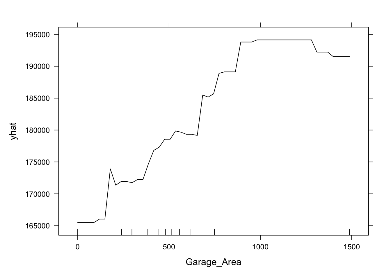
This nonlinear and complex relationship between Garage_Area and Sale_Price is similar to the plot we saw earlier with the GAMs and random forests. This shouldn’t be too surprising. All of these algorithms are trying to relate these two variables together, just in different ways.
In summary, XGBoost models are good models to use for prediction, but explanation becomes more difficult and complex. Some of the advantages of using XGBoost models:
Very accurate
Tend to outperform random forests when properly trained and tuned.
Variable importance provided
There are some disadvantages though:
“Interpretability” is a little different than the classical sense
Computationally slower than random forests due to sequentially building trees
More tuning parameters than random forests
Harder to optimize
More sensitive to tuning of parameters
A newer algorithm has come onto the scene that tries to have the predictive power seen in XGBoost models but maintain the kind of interpretability that GAM models have. This model is called the explainable boosting machine (EBM).
We covered GAM’s in the previous section, but as a reminder, GAM’s provide a general framework for the adding of non-linear functions together instead of the typical linear structure. The structure of GAM’s are the following:
\[ y = \beta_0 + f_1(x_1) + \cdots + f_p(x_p) + \varepsilon \]
The \(f_i(x_i)\) functions are complex, nonlinear functions on the predictor variables. GAM’s add these complex, yet individual functions together. This allows for many complex relationships to try and model with to potentially predict your target variable better.
EBM’s use machine learning algorithms (like random forests and boosting trees) to build these individual pieces, \(f_i (x_i)\), before adding them together in the GAM. To do this, they build out the same GBM structure but only use one variable at a time. The idea behind the GBM is to build a simple model to predict the target (much like a decision tree or even decision stump):
\[ y = g_1(x_1) + \varepsilon_1 \]
However, in the EBM that simple model is built only off of one variable, say \(x_1\). That simple model has an error of \(\varepsilon_1\). The next step is to try to predict that error with another simple model only using one other variable, say \(x_2\):
\[ \varepsilon_1 = g_2(x_2) + \varepsilon_2 \]
This model has an error of \(\varepsilon_2\). We can continue to add model after model, each one predicting the error (residuals) from the previous round, but only ever using one variable:
\[ y = g_1(x_1) + g_2(x_2) + \cdots + g_k(x_k) + \varepsilon_k \]
We will continue this process until we use all of the variables. We will then repeat this process in a round robin format, but still looking at the residuals from the previous set of models:
\[ y = g_1(x_1) + g_2(x_2) + \cdots + g_k(x_k) + \varepsilon_k \]
\[ \varepsilon_k = g_{1^*}(x_1) + g_{2^*}(x_2) + \cdots + g_{k^*}(x_k) + \varepsilon_{k^*} \]
\[ \varepsilon_{k^{*}} = g_{1^{**}}(x_1) + g_{2^{**}}(x_2) + \cdots + g_{k^{**}}(x_k) + \varepsilon_{k^{**}} \]
\[ \vdots \]
This will be repeated in a round robin format for thousands of iterations similar to a random forest approach where size of the iterations help find all the signal. We will apply a small learning rate to each of the subsequent models (each trees contribution to the running residual is scaled by a small number) so that the order of the variables will not matter. For each of the small models containing only the variable \(x_1\), \(g_1(x_1)\), \(g_{1^*}(x_1)\), \(g_{1^{**}}(x_1)\), etc. , we will aggregate them together to form our idea of the overall relationship between \(x_1\) and \(y\), our \(f_1(x_1)\) for our GAM:
\[ y = \beta_0 + f_1(x_1) + \cdots + f_p(x_p) + \varepsilon \]
We will then repeat this process for all of the variables in the model. Essentially, we are developing each of the pieces of the GAM (the individual variable relationships) and then adding them together to form our overall model.
These allow for individually developed relationships for variables which makes the interpretability more similar to that of the traditional GAM’s, but with the predictive power of the more advanced machine learning boosting algorithms.
Let’s see this in each of our softwares!
R has a newer implementation of the EBM model with the interpret package. However, that package will only apply the EBM model to a binary target variable. We will create a categorical target variable called Bonus that imagines homes selling for more than $175,000 nets the real estate agent a bonus. If Bonus takes a value of 1, the house sold for more than $175,000 and 0 otherwise.
ames <- ames %>%
  mutate(Bonus = ifelse(Sale_Price > 175000, 1, 0))

set.seed(4321)

training_c <- ames %>% sample_frac(0.7)
testing_c <- anti_join(ames, training_c, by = 'id')

training_c <- training_c %>%
  select(Bonus,
         Bedroom_AbvGr,
         Year_Built,
         Mo_Sold,
         Lot_Area,
         Street,
         Central_Air,
         First_Flr_SF,
         Second_Flr_SF,
         Full_Bath,
         Half_Bath,
         Fireplaces,
         Garage_Area,
         Gr_Liv_Area,
         TotRms_AbvGrd)
With the interpret package in R we have the ebm_classify function to model our Bonus variable we defined above. To build an EBM model we need separate data matrices for our predictors and our target variable. First we use the model.matrix function to create our predictor variable matrix. This will leave any continuous variables along and create any categorical dummy variables needed. We also isolate the target variable into its own vector. The predictor variable matrix and target variable vector will go into the X =and y = options in the ebm_classify function respectively.
library(interpret)

training_c_X <- model.matrix(Bonus ~ ., data = training_c)
training_c_Y <- training_c$Bonus

set.seed(1234)
ebm.model <- ebm_classify(X = training_c_X,
                          y = training_c_Y)
Python has a much more developed version of the EBM model than R does. It can build an EBM with either a continuous or categorical target variable. Let’s see examples of both.
First, we will try to predict our housing prices in Ames, Iowa as before. To do this we will use the interpret and interpret.glassbox packages and the ExplainableBoostingRegressor function. In the ExplainableBoostingRegressor function we limit the number of interactions we want to allow in the model. By default, this function will allow up to 90% of the count of variables as the number of possible interactions. Similar to other Python functions we have used, we need the training predictor variables in one object and the target variable in another. These will be passed to the .fit portion of the code below.
import interpret
from interpret.glassbox import ExplainableBoostingRegressor

ebm_model = ExplainableBoostingRegressor(interactions = 3)
ebm_model.fit(X_train, y_train)ExplainableBoostingRegressor(interactions=3)In a Jupyter environment, please rerun this cell to show the HTML representation or trust the notebook.
ExplainableBoostingRegressor(interactions=3)
To build a model similar to the one in the R portion of the code, we can create a categorical target variable called Bonus that imagines homes selling for more than $175,000 nets the real estate agent a bonus. If Bonus takes a value of 1, the house sold for more than $175,000 and 0 otherwise. This was created in R and imported here in Python to make sure we have the same training and testing observations.
training_c = r.training_c
testing_c = r.testing_c

import pandas as pd

train_dummy = pd.get_dummies(training_c, columns = ['Street', 'Central_Air'])

y_train_c = train_dummy['Bonus']

X_train_c = train_dummy.loc[:, train_dummy.columns != 'Bonus']
Since we have a categorical target variable instead, we will use the ExplainableBoostingClassifier function. In the ExplainableBoostingClassifier function we limit the number of interactions we want to allow in the model. By default, this function will allow up to 90% of the count of variables as the number of possible interactions. Similar to other Python functions we have used, we need the training predictor variables in one object and the target variable in another. These will be passed to the .fit portion of the code below.
from interpret.glassbox import ExplainableBoostingClassifier

ebm_model_c = ExplainableBoostingClassifier(interactions = 3)
ebm_model_c.fit(X_train_c, y_train_c)ExplainableBoostingClassifier(interactions=3)In a Jupyter environment, please rerun this cell to show the HTML representation or trust the notebook.
ExplainableBoostingClassifier(interactions=3)
Now we have an EBM model built. We can use some of the functionality of that model to try and interpret the variables. Remember the GAM structure to the EBM as described above. This allows for individually developed relationships for variables which makes the interpretability more similar to that of the traditional GAM’s, but with the predictive power of the more advanced machine learning boosting algorithms.
Let’s see this in each of our softwares!
In R, we use the ebm_show function to allow us to visualize the individual relationships from our EBM model. The inputs to the ebm_show function are the EBM model object along with the name of the variable of interest. Here we will use the Garage_Area variable.
ebm_show(ebm.model, "Garage_Area")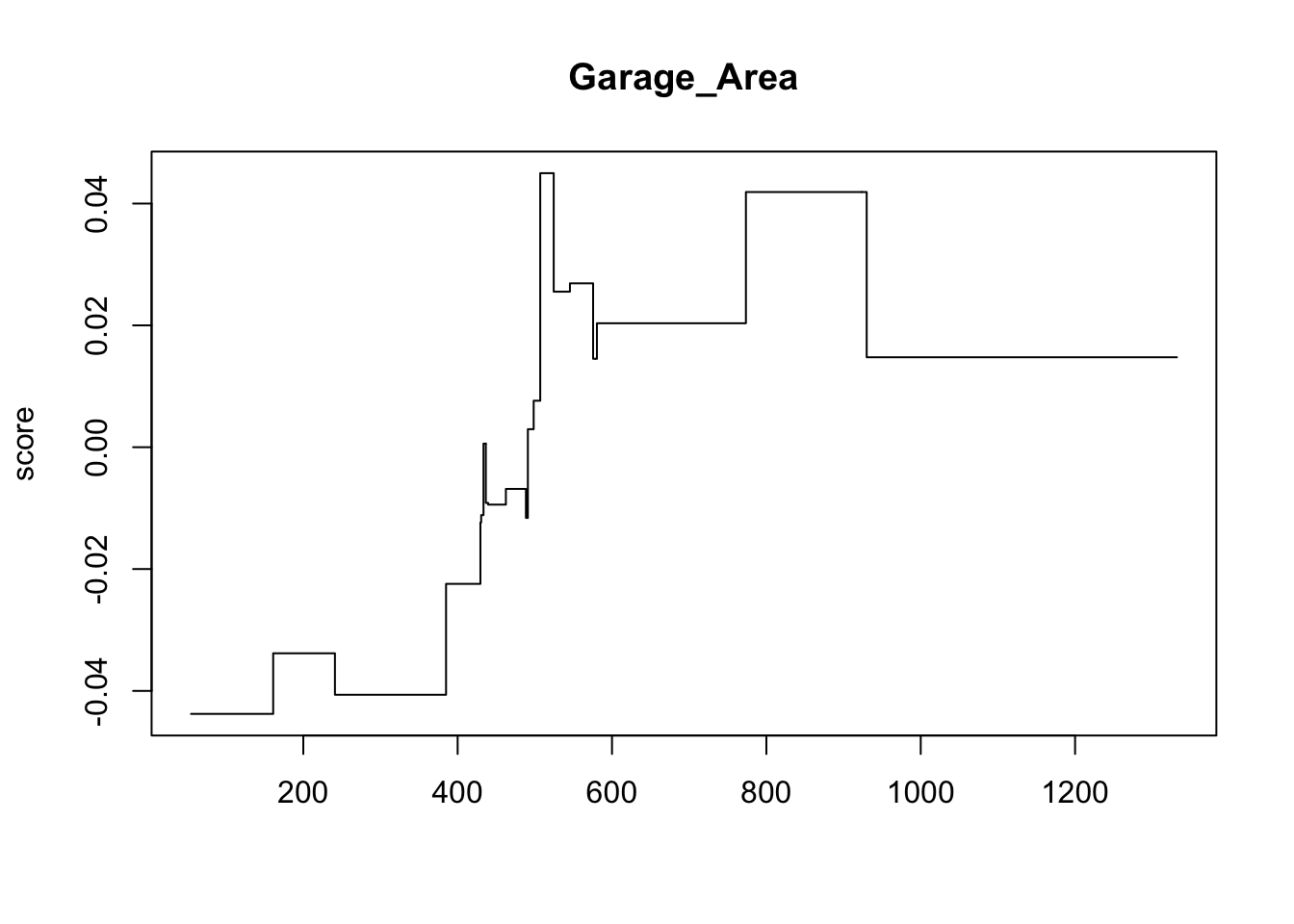
This nonlinear and complex relationship between Garage_Area and Sale_Price is similar to the plot we saw earlier with the GAMs, random forests, and XGBoost models. This shouldn’t be too surprising. All of these algorithms are trying to relate these two variables together, just in different ways.
Similar to the model development, Python has a more robust set of interpretations for the EBM model compared to R. From the interpret package we will need the show, InlineProvider, and set_visualize_provider functions. First, we use the set_visualize_provider function with the InlineProvider function to scan our environment and use the best visualization setup for our environment. From there we can start to visualize the model features.
First, we will use the explain_global() function on the EBM model object created above. This will calculate all of the global interpretations from our model. From there we can use the visualize() function as well as the show function to plot the global importance.
from interpret import show
from interpret.provider import InlineProvider
from interpret import set_visualize_provider

set_visualize_provider(InlineProvider())

ebm_global = ebm_model.explain_global()

plotly_fig = ebm_global.visualize()

plotly_fig.show()
From the plot above we have a global importance score for each variable. Let’s look at the first variable, Year_Built. This variable has a weighted Mean Absolute Score of 22,878. This has some interpretive value! This means that, on average, the Year_Built variable moved predictions in some direction by $22,878. This average movement was larger than any other variable in terms of impact. We can see the same thing for the remaining variables.
If we wanted to explore the variables on an individual level we can call a specific variable by number in the visualize function as shown below. The variables are listed in the order they are put into the model, however, the continuous variables are all grouped first, followed by the categorical variables. For example, the Garage_Area variable is the 10th (index value of 9) continuous predictor variable put in our model.
ebm_global = ebm_model.explain_global()

plotly_fig = ebm_global.visualize(9)

plotly_fig.show()
From the plot above we can see the predicted relationship between the variable Garage_Area and Sale_Price. This nonlinear and complex relationship is similar to the plot we saw earlier with the GAMs, random forests, and XGBoost models. This shouldn’t be too surprising. All of these algorithms are trying to relate these two variables together, just in different ways. The density plot below this graph is just a histogram of the values of Garage_Area.
For completeness sake, below is the same code, but for the EBM model built on our binary target variable of Bonus. First, we will use the explain_global() function on the EBM model object created above. This will calculate all of the global interpretations from our model. From there we can use the visualize() function as well as the show function to plot the global importance.
ebm_global_c = ebm_model_c.explain_global()

plotly_fig_c = ebm_global_c.visualize()

plotly_fig_c.show()
From the plot above we have a global importance score for each variable. Let’s look at the first variable, Year_Built. This variable has a weighted Mean Absolute Score of 1.379. Unlike with the continuous target variable, this doesn’t have as nice of an interpretation. This means that, on average, the Year_Built variable moved the natural log of the odds (logit) in some direction by 1.379. This average movement was larger than any other variable in terms of impact. We can see the same thing for the remaining variables.
If we wanted to explore the variables on an individual level we can call a specific variable by number in the visualize function as shown below. The variables are listed in the order they are put into the model, however, the continuous variables are all grouped first, followed by the categorical variables. For example, the Garage_Area variable is the 10th (index value of 9) continuous predictor variable put in our model.
ebm_global_c = ebm_model_c.explain_global()

plotly_fig = ebm_global_c.visualize(9)

plotly_fig.show()Another thing to tune would be which variables to include in the EBM model. By default, EBM models use all the variables since they are aggregated across all the trees used to build the model. There are a couple of ways to perform variable selection for XGBoost:
Many permutations of including/excluding variables
Compare variables to random variable
The first approach is rather straight forward but time consuming because you have to try and build models over and over again taking a variable out each time. The second approach is much easier to try. In that second approach we will create a completely random variable and put it in the model. We will then look at the variable importance of all the variables. The variables that are below the random variable should be considered for removal.
To create a random variable in Python we will first create a new data.frame called X_train_r. We will then add a variable called random with the random.normal function from numpy. We then build an EBM model in the same way we did previously and check the variable importance.
import numpy as np

X_train_r = X_train

X_train_r['random'] = np.random.normal(0, 1, 2051)
Instead of plotting the variable importance for the variables we will just print out a list of the importance for each variable using the term_importance and term_name functions.
ebm_model_r = ExplainableBoostingRegressor(interactions = 3)
ebm_model_r.fit(X_train_r, y_train)ExplainableBoostingRegressor(interactions=3)In a Jupyter environment, please rerun this cell to show the HTML representation or trust the notebook.
ExplainableBoostingRegressor(interactions=3)
importances = ebm_model_r.term_importances()
names = ebm_model_r.term_names_

for (term_name, importance) in zip(names, importances):
    print(f"Term {term_name} importance: {importance}")
Term Bedroom_AbvGr importance: 4901.041451211291
Term Year_Built importance: 22997.063116381727
Term Mo_Sold importance: 1329.0039429978642
Term Lot_Area importance: 4280.288354408339
Term First_Flr_SF importance: 15515.769369838674
Term Second_Flr_SF importance: 5233.633411745021
Term Full_Bath importance: 1715.0167905473766
Term Half_Bath importance: 4084.5149261854303
Term Fireplaces importance: 8253.832541813987
Term Garage_Area importance: 7714.547082485783
Term Gr_Liv_Area importance: 13999.799248736503
Term TotRms_AbvGrd importance: 1593.4741727639848
Term Street_Grvl importance: 80.83097345516985
Term Street_Pave importance: 80.19763190781755
Term Central_Air_N importance: 1300.637422295222
Term Central_Air_Y importance: 1324.8608978376571
Term random importance: 1221.323581228066
Term Year_Built & First_Flr_SF importance: 4643.669492471417
Term Year_Built & Garage_Area importance: 2360.574748076047
Term Year_Built & Gr_Liv_Area importance: 2664.716971831796Based on the list above there are 3 variables that fall below the variable importance of the random variable that could be considered for removal from the model.
Another valuable piece of output from the Python functionality of EBM models is the ability to perform local interpretability as well as the global interpretability we saw earlier.
ebm_local = ebm_model.explain_local(X_train[:1], y_train[:1])

plotly_fig = ebm_local.visualize(0)

plotly_fig.show()
The above plot breaks down the individual prediction from the model into how each variable impacts prediction. More details on these kinds of calculations are listed in the Model Agnostic Interpretability section of the notes.
In summary, EBM models are good models to use for prediction and keeps similar interpretability of GAM models. Some of the advantages of using EBM models:
Early results show they are powerful at predicting (almost to the level of XGBoost).
Interpretation available due to GAM nature (individually estimated relationships)
There are some disadvantages though:
Computationally slower than random forests due to sequentially building trees
More tuning parameters than random forests
Limited implementations across all softwares