Neural network models are considered “black-box” models because they are complex and hard to decipher relationships between predictor variables and the target variable. However, if the focus is on prediction, these models have the potential to model very complicated patterns in data sets with either continuous or categorical targets.
The concept of neural networks was well received back in the 1980’s. However, it didn’t live up to expectations. Support vector machines (SVM’s) overtook neural networks in the early 2000’s as the popular “black-box” model. Recently there has been a revitalized growth of neural network models in image and visual recognition problems. There is now a lot of research in the area of neural networks and “deep learning” problems - recurrent, convolutional, feedforward, etc.
Neural networks were originally proposed as a structure to mimic the human brain. We have since found out that the human brain is much more complex. However, the terminology is still the same. Neural networks are organized in a network of neurons (or nodes) through layers. The input variables are considered the neurons on the bottom layer. The output variable is considered the neuron on the top layer. The layers in between, called hidden layers, transform the input variables through non-linear methods to try and best model the output variable.
Single Hidden Layer Neural Network
All of the nonlinearities and complication of the variables get added to the model in the hidden layer. Each line in the above figure is a weight that connects one layer to the next and needs to be optimized. For example, the first variable \(x_1\) is connected to all of the neurons (nodes) in the hidden layer with a separate weight.
Let’s look in more detail about what is happening inside the first neuron of the hidden layer.
Each of the variables is weighted coming into the neuron. These weights are combined with each of the variables in a linear combination with each other. With the linear combination we then perform a non-linear transformation.
There are many different nonlinear functions this could be. The main goal is to add complexity to the model. Each of the hidden nodes apply different weights to each of the input variables. This would mean that certain nonlinear relationships are highlighted for certain variables more than others. This is why we can have lots of neurons in the hidden layer so that many nonlinear relationships can be built.
From there, each of the hidden layer neurons passes this nonlinear transformation to the next layer. If that next layer is another hidden layer, then the nonlinear transformations from each neuron in the first hidden layer are combined linearly in a weighted combination and another nonlinear transformation is applied to them. If the output layer is the next layer, then these nonlinear transformations are combined linearly in a weighted combination for a last time.
Now we have the final prediction from our model. All of the weights that we have collected along the way are optimized to minimize sum of squared error. How this optimization is done is through a process called backpropagation.
Backpropagation
Backpropagation is the process that is used to optimize the coefficients (weights) in the neural network. There are two main phases to backpropagation - a forward and backward phase.
In the forward phase we have the following steps:
Start with some initial weights (often random)
Calculations pass through the network
Predicted value computed.
In the backward phase we have the following steps:
Predicted value compared with actual value
Work backward through the network to adjust weights to make the prediction better
Repeat forward and backward until process converges
Let’s look at a basic example with 3 neurons in the input layer, 2 neurons in the hidden layer, and one neuron in the output layer.
Imagine 3 variables that take the values of 3, 4, and 5 with the corresponding weights being assigned to each line in the graph above. For the top neuron in the hidden layer you have \(3\times 1 + 4 \times 0 + 5 \times 1 = 8\). The same process can be taken to get the bottom neuron. The hidden layer node values are then combined together (with no nonlinear transformation here) together to get the output layer.
For the backward phase of backpropagation, let’s imagine the true value of the target variable for this observation was 34. That means we have an error of 6 (\(34-28=6\)). We will now work our way back through the network changing the weights to make this prediction better. To see this process, let’s use an even simpler example.
Imagine you have a very simple equation, \(y = \beta_1 x\). Now let’s imagine you know that \(y = 20\) and \(x = 5\). However, you forgot how to do division! So you need backpropagation to find the value of \(\beta_1\). To start with the forward phase, let’s just randomly guess 3 for \(\beta_1\) - our random starting point. Going through the network, we will use this guess of \(\beta_1\) to get our final prediction of 15 (\(=3 \times 5\)). Since we know the true value of y is 20, we start with an error of \(20-15 = 5\). Now we look at the backward phase of backpropagation. First we need the derivative of our loss function (sum of squared error). Without going through all the calculus details here, the derivative of the squared error at a single point is 2 multiplied by the error itself.
The next step in baackpropagation is to adjust our original value of \(\beta_1\) to account for this error and get a better estimate of \(\beta_1\). To do this we multiply the slope of the error curve by the learning rate (set at some small constant like 0.05 to start) and then adjust the value of \(\beta_1\).
Based on the figure above, our \(\beta_1\) was 3, but has been adjusted to 3.5 based on the learning rate and slope of the loss function. Now we repeat the process and go forward through the network. This makes our prediction 17.5 instead of 15. This reduces our error from 5 to 2.5. The process goes backwards again to adjust the value of \(\beta_1\) again.
We will still multiply the slope of the loss function (with our new error) by the learning rate. This learning rate should be adjusted to be smaller (from 0.05 to 0.04 above) to account for us being closer to the real answer. We will not detail how the backpropagation algorithm adjusts this learning rate here. However, this process will continue until some notion of convergence. In this example, it would continue until the slope estimate is 4 and the error would be 0 (its minimum).
Although easy in idea, in practice this is much more complicated. To start, we have many more than just one single observation. So we have to calculate the error of all of the observations and get a notion of our loss function (sum of squared error in our example) across all the observations. The changing of the slope then impacts all of the observations, not just a single one. Next, we have more than one variable and weight to optimize at each step, making the process all the more complicated. Finally, this gets even more complicated as we add in many neurons in hidden layers so the algorithm has many layers to step backward through in its attempt to optimize the solution. These hidden layers also have complicated nonlinear functions, which make derivative calculations much more complicated than the simple example we had above. Luckily, this is what the computer helps do for us!
Fitting a Neural Network
Let’s see how to build a neural network in each of our softwares!
Although not required, neural networks work best when data is scaled to a narrow range around 0. For bell shaped data, statistical z-score standardization would work:
\[
z_i = \frac{x_i-\bar{x}}{s_x}
\]
For severely asymmetric data, midrange standardization works better:
For simplicity, we will use the scale function to standardize our data with the z-score method.
Code
training <- training %>%mutate(s_Bedroom_AbvGr =scale(Bedroom_AbvGr),s_Year_Built =scale(Year_Built),s_Mo_Sold =scale(Mo_Sold),s_Lot_Area =scale(Lot_Area),s_First_Flr_SF =scale(First_Flr_SF),s_Second_Flr_SF =scale(Second_Flr_SF),s_Garage_Area =scale(Garage_Area),s_Gr_Liv_Area =scale(Gr_Liv_Area),s_TotRms_AbvGrd =scale(TotRms_AbvGrd))training$Full_Bath <-as.factor(training$Full_Bath)training$Half_Bath <-as.factor(training$Half_Bath)training$Fireplaces <-as.factor(training$Fireplaces)
We will then use the nnet and NeuralNetTools packages to build out our neural network. The nnet function has typical inputs. First we need our formula, which now has the scaled version of our continuous variables. The size = option specifies how many neurons we want in the hidden layer. The nnet function can only build single hidden layer neural networks. The linout option specifies the linear output instead of a logistic output.
# weights:  116
initial  value 79865940344074.140625
iter  10 value 7099497202797.828125
iter  20 value 6636275639715.039062
final  value 6617571512706.858398
converged
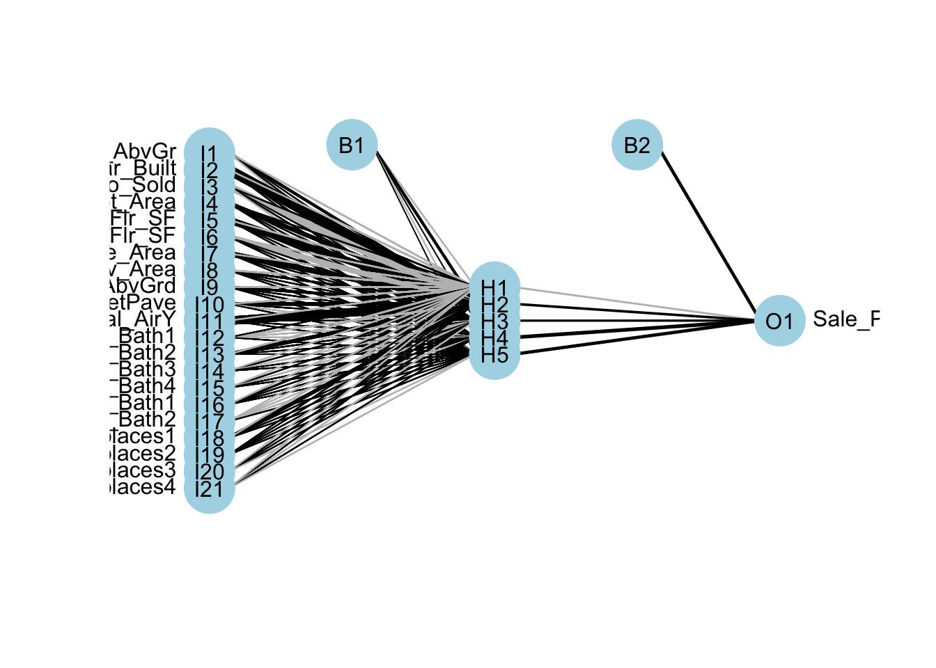
If you are curious in looking at the network, we can always plot the model object with the plot function.
Code
plotnet(nn.ames)
The downside of the nnet function is the lack of tuning ability. Again, we will go to the train function from caret to help. In the expand.grid for this iteration of the train function we will use the .size and .decay parameters. The .size parameter controls how many neurons are in our single hidden layer. We will try out values of 3 through 7. The .decay parameter is a regularization parameter to prevent overfitting. We will use the bestTune element from the model object to see the optimal values of the parameters.
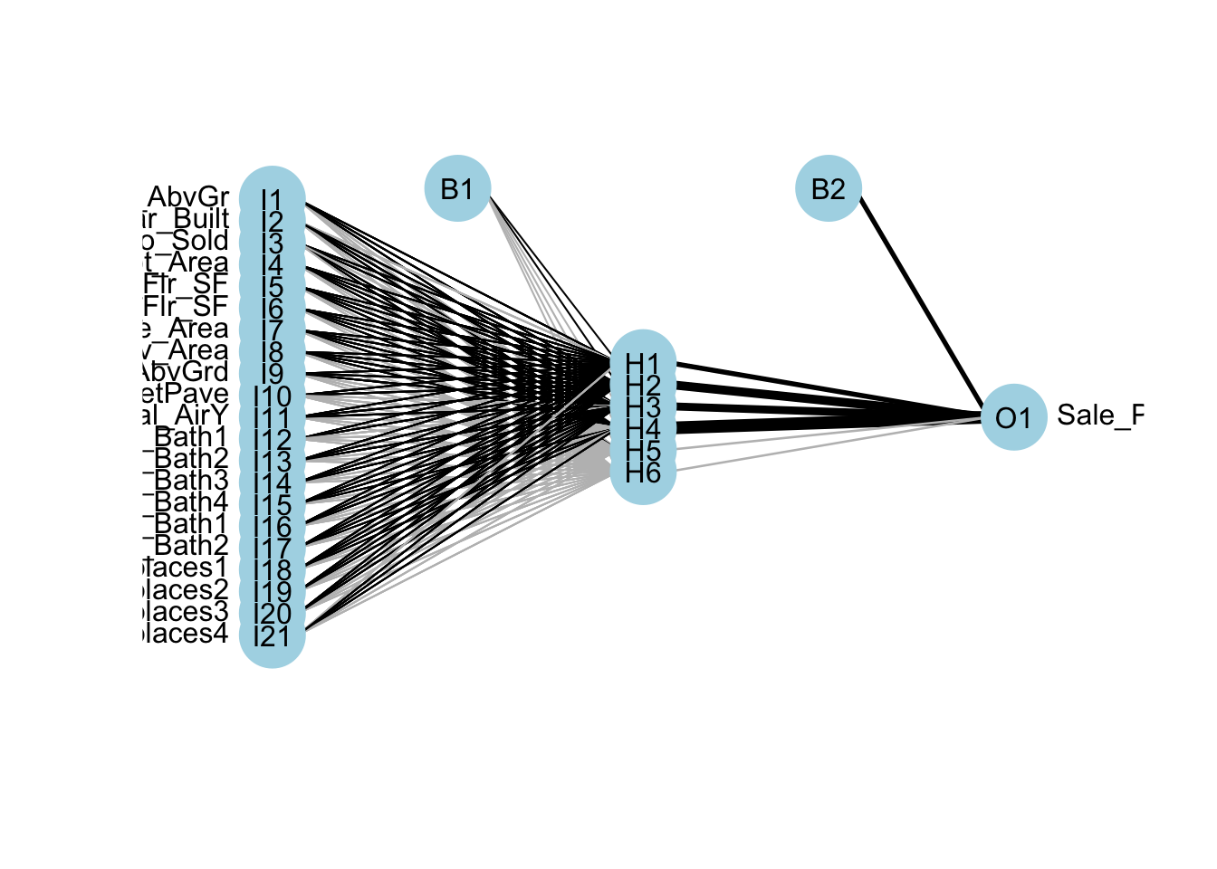
From the output above it seems like the neural network is optimized with 7 neurons in the hidden layer and a decay factor of 1. We can put these back into our original model if we like to better view them with the plot function.
# weights:  162
initial  value 79866178455117.750000
iter  10 value 6821832280076.744141
iter  20 value 6149226099997.672852
iter  30 value 6092474606530.930664
iter  40 value 6059418519235.842773
iter  50 value 6037089307201.352539
iter  60 value 6026416194356.576172
iter  70 value 5950160210126.250977
iter  80 value 5476715254389.529297
iter  90 value 5358516839487.140625
iter 100 value 5334489488905.238281
final  value 5334489488905.238281
stopped after 100 iterations
Code
plotnet(nn.ames)
Although not required, neural networks work best when data is scaled to a narrow range around 0. For bell shaped data, statistical z-score standardization would work:
\[
z_i = \frac{x_i - \bar{x}}{s_x}
\]
For severely asymmetric data, midrange standardization works better:
For simplicity, we will use the StandardScaler function to standardize our data with the z-score method.
Code
from sklearn.preprocessing import StandardScaler

scaler = StandardScaler()
scaler.fit(X = X_train)
StandardScaler()
In a Jupyter environment, please rerun this cell to show the HTML representation or trust the notebook. On GitHub, the HTML representation is unable to render, please try loading this page with nbviewer.org.
StandardScaler()
Code
X_train_s = scaler.transform(X_train)
We will then use the MLPRegressor function from the sklearn.neural_network packages to build out our neural network. The MLPRegressor function has expected inputs. The hidden_layer_sizes = option specifies how many neurons we want in each hidden layer. For multiple hidden layers, you would put multiple numbers. We will build one hidden layer with 5 neurons. We then use the .fit function with our standardized predictors and target variable to build out our model.
In a Jupyter environment, please rerun this cell to show the HTML representation or trust the notebook. On GitHub, the HTML representation is unable to render, please try loading this page with nbviewer.org.
The downside of the MLPRegressor function is the lack of tuning ability. Again, we will go to the GridSearchCV function from sklearn.model_selection to help. In the param_grid for this iteration of the GridSearchCV function we will use the hidden_layer_sizes, alpha, and solver parameters. The hidden_layer_sizes parameter controls how many neurons are in our hidden layer. We will try out values of 3 through 7. The alpha parameter is a regularization parameter to prevent overfitting. We will leave the solver parameter alone and not worry about trying different optimization techniques. We will still keep our usual 10-fold cross-validation.
In a Jupyter environment, please rerun this cell to show the HTML representation or trust the notebook. On GitHub, the HTML representation is unable to render, please try loading this page with nbviewer.org.
We can see that having 4 neurons in our hidden layer with an alpha parameter of 0.0003 is the optimal solution.
Variable Selection
Neural networks typically do not care about variable selection. All variables are used by default in a complicated and mixed way. However, if you want to do variable selection, you can examine the weights for each variable. If all of the weights for a single variable are low, then you might consider deleting the variable, but again, it is typically not required.
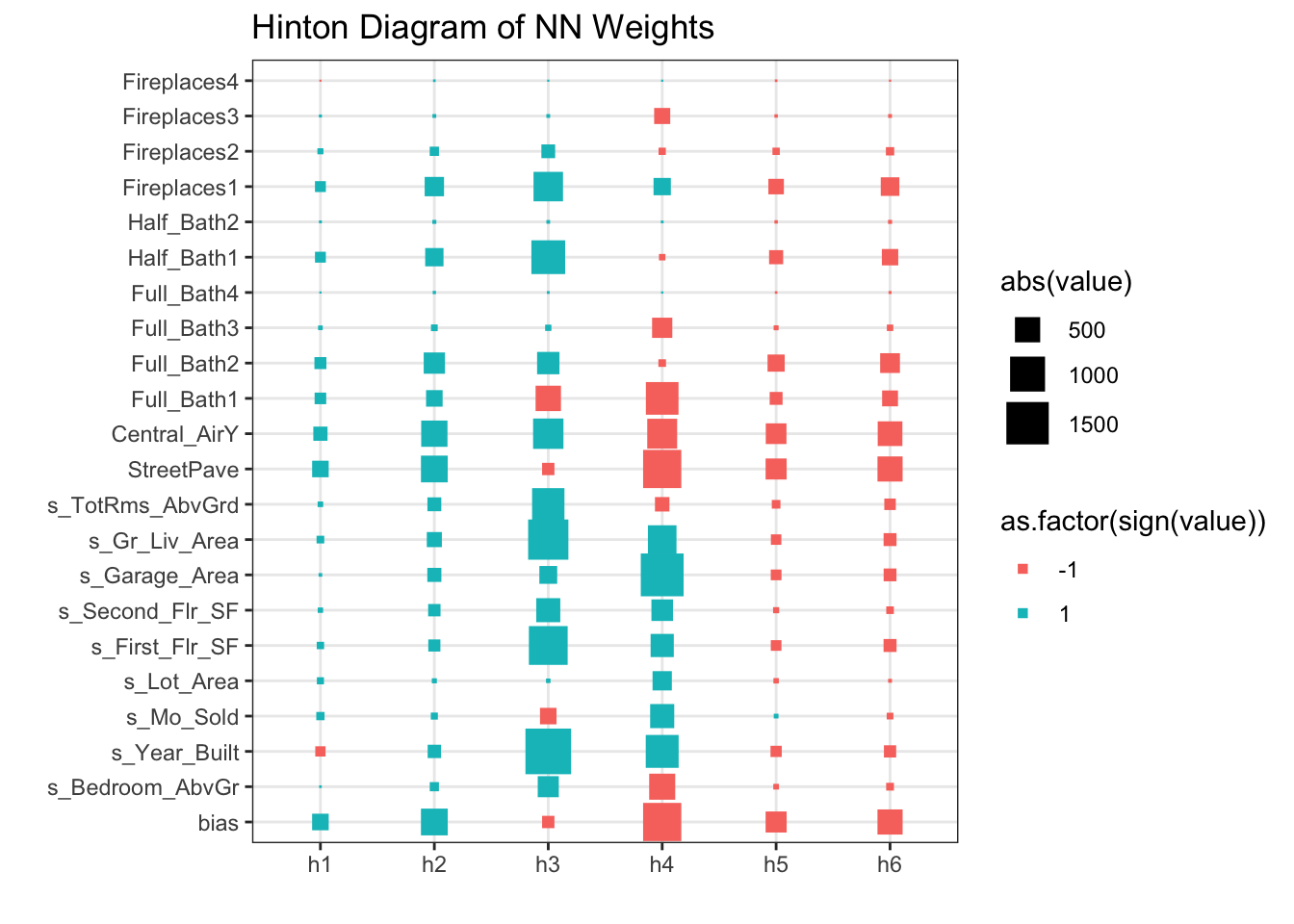
One way to visualize all the weights in a variable would be to use a Hinton diagram. This diagram is really only good for smaller numbers of variables. With hundreds of variables, a Hinton diagram becomes burdensome to view.
Code
library(ggplot2)library(reshape2)nn_weights <-matrix(data = nn.ames$wts[1:132], ncol =22, nrow =6, byrow =TRUE)colnames(nn_weights) <-c("bias", nn.ames$coefnames)rownames(nn_weights) <-c("h1", "h2", "h3", "h4", "h5", "h6")ggplot(melt(nn_weights), aes(x=Var1, y=Var2, size=abs(value), color=as.factor(sign(value)))) +geom_point(shape =15) +scale_size_area(max_size =8) +labs(x ="", y ="", title ="Hinton Diagram of NN Weights") +theme_bw()
From the diagram above we see there are few instances of variables having low weights across all of the inputs to the hidden layers. The only ones we see are specific categories in a larger categorical variable. In this scenario, we would probably keep all of our variables.
Summary
In summary, neural network models are good models to use for prediction, but explanation becomes more difficult and complex. Some of the advantages of using neural network models:
Used for both categorical and numeric target variables
Capable of modeling complex, nonlinear patterns
No assumptions about the data distributions
There are some disadvantages though:
No insights for variable importance
Extremely computationally intensive (very slow to train)
Tuning of parameters is burdensome
Prone to overfitting training data
Source Code
---title: "Neural Network Models"format: html: code-fold: show code-tools: trueeditor: visual---```{r}#| include: false#| warning: false#| error: false#| message: falselibrary(AmesHousing)ames <-make_ordinal_ames()library(tidyverse)ames <- ames %>%mutate(id =row_number())set.seed(4321)training <- ames %>%sample_frac(0.7)testing <-anti_join(ames, training, by ='id')training <- training %>%select(Sale_Price, Bedroom_AbvGr, Year_Built, Mo_Sold, Lot_Area, Street, Central_Air, First_Flr_SF, Second_Flr_SF, Full_Bath, Half_Bath, Fireplaces, Garage_Area, Gr_Liv_Area, TotRms_AbvGrd)``````{python}#| include: false#| warning: false#| error: false#| message: falsetraining = r.trainingtesting = r.testingimport pandas as pdtrain_dummy = pd.get_dummies(training, columns = ['Street', 'Central_Air'])print(train_dummy)y_train = train_dummy['Sale_Price']X_train = train_dummy.loc[:, train_dummy.columns !='Sale_Price']```# Neural Network StructureNeural network models are considered "black-box" models because they are complex and hard to decipher relationships between predictor variables and the target variable. However, if the focus is on prediction, these models have the potential to model very complicated patterns in data sets with either continuous or categorical targets.The concept of neural networks was well received back in the 1980's. However, it didn't live up to expectations. Support vector machines (SVM's) overtook neural networks in the early 2000's as the popular "black-box" model. Recently there has been a revitalized growth of neural network models in image and visual recognition problems. There is now a lot of research in the area of neural networks and "deep learning" problems - recurrent, convolutional, feedforward, etc.Neural networks were originally proposed as a structure to mimic the human brain. We have since found out that the human brain is much more complex. However, the terminology is still the same. Neural networks are organized in a network of **neurons** (or nodes) through **layers**. The input variables are considered the neurons on the **bottom layer**. The output variable is considered the neuron on the **top layer**. The layers in between, called **hidden layers**, transform the input variables through non-linear methods to try and best model the output variable.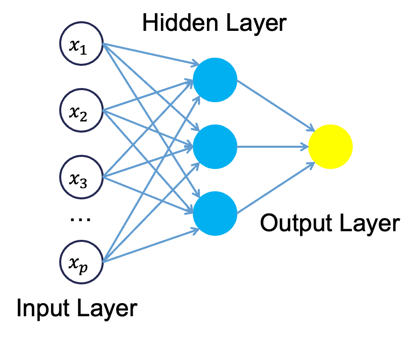{fig-align="center" width="4in"}All of the nonlinearities and complication of the variables get added to the model in the hidden layer. Each line in the above figure is a weight that connects one layer to the next and needs to be optimized. For example, the first variable $x_1$ is connected to all of the neurons (nodes) in the hidden layer with a separate weight.Let's look in more detail about what is happening inside the first neuron of the hidden layer.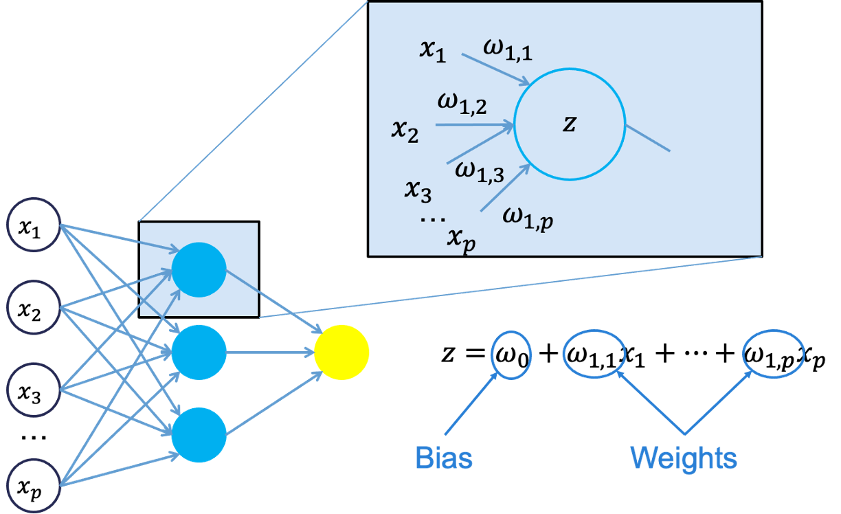{fig-align="center" width="7in"}Each of the variables is weighted coming into the neuron. These weights are combined with each of the variables in a linear combination with each other. With the linear combination we then perform a non-linear transformation.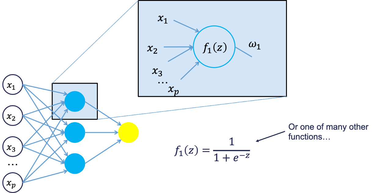{fig-align="center" width="7in"}There are many different nonlinear functions this could be. The main goal is to add complexity to the model. Each of the hidden nodes apply different weights to each of the input variables. This would mean that certain nonlinear relationships are highlighted for certain variables more than others. This is why we can have lots of neurons in the hidden layer so that many nonlinear relationships can be built.From there, each of the hidden layer neurons passes this nonlinear transformation to the next layer. If that next layer is another hidden layer, then the nonlinear transformations from each neuron in the first hidden layer are combined linearly in a weighted combination and another nonlinear transformation is applied to them. If the output layer is the next layer, then these nonlinear transformations are combined linearly in a weighted combination for a last time.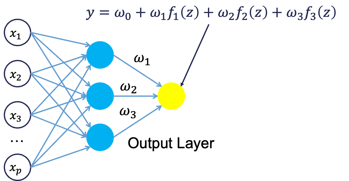{fig-align="center" width="5in"}Now we have the final prediction from our model. All of the weights that we have collected along the way are optimized to minimize sum of squared error. How this optimization is done is through a process called **backpropagation**.# BackpropagationBackpropagation is the process that is used to optimize the coefficients (weights) in the neural network. There are two main phases to backpropagation - a forward and backward phase.In the forward phase we have the following steps:1. Start with some initial weights (often random)2. Calculations pass through the network3. Predicted value computed.In the backward phase we have the following steps:1. Predicted value compared with actual value2. Work backward through the network to adjust weights to make the prediction better3. Repeat forward and backward until process convergesLet's look at a basic example with 3 neurons in the input layer, 2 neurons in the hidden layer, and one neuron in the output layer.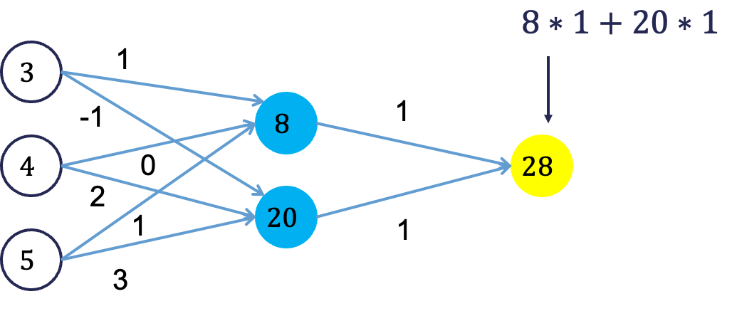{fig-align="center" width="5in"}Imagine 3 variables that take the values of 3, 4, and 5 with the corresponding weights being assigned to each line in the graph above. For the top neuron in the hidden layer you have $3\times 1 + 4 \times 0 + 5 \times 1 = 8$. The same process can be taken to get the bottom neuron. The hidden layer node values are then combined together (with no nonlinear transformation here) together to get the output layer.For the backward phase of backpropagation, let's imagine the true value of the target variable for this observation was 34. That means we have an error of 6 ($34-28=6$). We will now work our way back through the network changing the weights to make this prediction better. To see this process, let's use an even simpler example.Imagine you have a very simple equation, $y = \beta_1 x$. Now let's imagine you know that $y = 20$ and $x = 5$. However, you forgot how to do division! So you need backpropagation to find the value of $\beta_1$. To start with the forward phase, let's just randomly guess 3 for $\beta_1$ - our random starting point. Going through the network, we will use this guess of $\beta_1$ to get our final prediction of 15 ($=3 \times 5$). Since we know the true value of y is 20, we start with an error of $20-15 = 5$. Now we look at the backward phase of backpropagation. First we need the derivative of our loss function (sum of squared error). Without going through all the calculus details here, the derivative of the squared error at a single point is 2 multiplied by the error itself.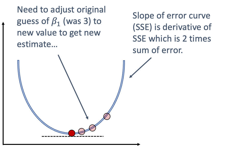{fig-align="center" width="5in"}The next step in baackpropagation is to adjust our original value of $\beta_1$ to account for this error and get a better estimate of $\beta_1$. To do this we multiply the slope of the error curve by the learning rate (set at some small constant like 0.05 to start) and then adjust the value of $\beta_1$.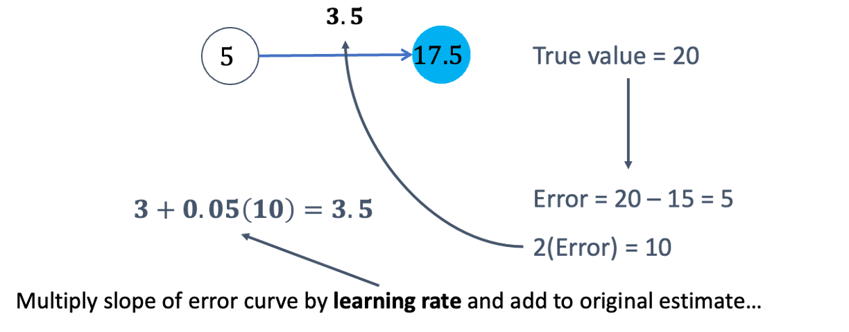{fig-align="center" width="6.5in"}Based on the figure above, our $\beta_1$ was 3, but has been adjusted to 3.5 based on the learning rate and slope of the loss function. Now we repeat the process and go forward through the network. This makes our prediction 17.5 instead of 15. This reduces our error from 5 to 2.5. The process goes backwards again to adjust the value of $\beta_1$ again.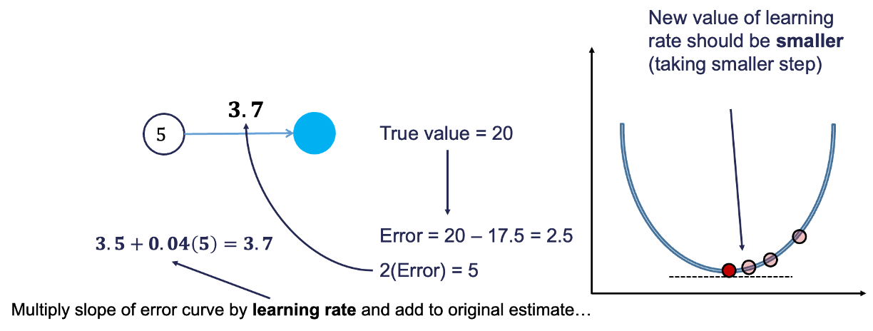{fig-align="center" width="8in"}We will still multiply the slope of the loss function (with our new error) by the learning rate. This learning rate should be adjusted to be smaller (from 0.05 to 0.04 above) to account for us being closer to the real answer. We will not detail how the backpropagation algorithm adjusts this learning rate here. However, this process will continue until some notion of convergence. In this example, it would continue until the slope estimate is 4 and the error would be 0 (its minimum).Although easy in idea, in practice this is much more complicated. To start, we have many more than just one single observation. So we have to calculate the error of all of the observations and get a notion of our loss function (sum of squared error in our example) across all the observations. The changing of the slope then impacts all of the observations, not just a single one. Next, we have more than one variable and weight to optimize at each step, making the process all the more complicated. Finally, this gets even more complicated as we add in many neurons in hidden layers so the algorithm has many layers to step backward through in its attempt to optimize the solution. These hidden layers also have complicated nonlinear functions, which make derivative calculations much more complicated than the simple example we had above. Luckily, this is what the computer helps do for us!# Fitting a Neural NetworkLet's see how to build a neural network in each of our softwares!::: {.panel-tabset .nav-pills}## RAlthough not required, neural networks work best when data is scaled to a narrow range around 0. For bell shaped data, statistical z-score standardization would work:$$z_i = \frac{x_i-\bar{x}}{s_x}$$For severely asymmetric data, midrange standardization works better:$$\frac{x_i - midrange(x)}{0.5 \times range(x)} = \frac{x_i -\frac{\max(x)+\min(x)}{2}}{0.5 \times (\max(x) - \min(x))}$$For simplicity, we will use the `scale` function to standardize our data with the z-score method.```{r}#| warning: false#| error: false#| message: falsetraining <- training %>%mutate(s_Bedroom_AbvGr =scale(Bedroom_AbvGr),s_Year_Built =scale(Year_Built),s_Mo_Sold =scale(Mo_Sold),s_Lot_Area =scale(Lot_Area),s_First_Flr_SF =scale(First_Flr_SF),s_Second_Flr_SF =scale(Second_Flr_SF),s_Garage_Area =scale(Garage_Area),s_Gr_Liv_Area =scale(Gr_Liv_Area),s_TotRms_AbvGrd =scale(TotRms_AbvGrd))training$Full_Bath <-as.factor(training$Full_Bath)training$Half_Bath <-as.factor(training$Half_Bath)training$Fireplaces <-as.factor(training$Fireplaces)```We will then use the `nnet` and `NeuralNetTools` packages to build out our neural network. The `nnet` function has typical inputs. First we need our formula, which now has the scaled version of our continuous variables. The `size =` option specifies how many neurons we want in the hidden layer. The `nnet` function can only build single hidden layer neural networks. The `linout` option specifies the linear output instead of a logistic output.```{r}#| warning: false#| error: false#| message: falselibrary(nnet)library(NeuralNetTools)set.seed(12345)nn.ames <-nnet(Sale_Price ~ s_Bedroom_AbvGr + s_Year_Built + s_Mo_Sold + s_Lot_Area + s_First_Flr_SF + s_Second_Flr_SF + s_Garage_Area + s_Gr_Liv_Area + s_TotRms_AbvGrd + Street + Central_Air + Full_Bath + Half_Bath + Fireplaces , data = training, size =5, linout =TRUE)```If you are curious in looking at the network, we can always plot the model object with the `plot` function.```{r}#| warning: false#| error: false#| message: falseplotnet(nn.ames)```The downside of the `nnet` function is the lack of tuning ability. Again, we will go to the `train` function from `caret` to help. In the `expand.grid` for this iteration of the `train` function we will use the `.size` and `.decay` parameters. The `.size` parameter controls how many neurons are in our single hidden layer. We will try out values of 3 through 7. The `.decay` parameter is a regularization parameter to prevent overfitting. We will use the `bestTune` element from the model object to see the optimal values of the parameters.```{r}#| warning: false#| error: false#| message: falselibrary(caret)tune_grid <-expand.grid(.size =c(3, 4, 5, 6, 7),.decay =c(0, 0.5, 1))set.seed(12345)nn.ames.caret <- caret::train(Sale_Price ~ s_Bedroom_AbvGr + s_Year_Built + s_Mo_Sold + s_Lot_Area + s_First_Flr_SF + s_Second_Flr_SF + s_Garage_Area + s_Gr_Liv_Area + s_TotRms_AbvGrd + Street + Central_Air + Full_Bath + Half_Bath + Fireplaces , data = training,method ="nnet", tuneGrid = tune_grid,trControl =trainControl(method ='cv', number =10),trace =FALSE, linout =TRUE)nn.ames.caret$bestTune```From the output above it seems like the neural network is optimized with 7 neurons in the hidden layer and a decay factor of 1. We can put these back into our original model if we like to better view them with the `plot` function.```{r}#| warning: false#| error: false#| message: falseset.seed(12345)nn.ames <-nnet(Sale_Price ~ s_Bedroom_AbvGr + s_Year_Built + s_Mo_Sold + s_Lot_Area + s_First_Flr_SF + s_Second_Flr_SF + s_Garage_Area + s_Gr_Liv_Area + s_TotRms_AbvGrd + Street + Central_Air + Full_Bath + Half_Bath + Fireplaces , data = training, size =7, decay =0.5, linout =TRUE)plotnet(nn.ames)```## PythonAlthough not required, neural networks work best when data is scaled to a narrow range around 0. For bell shaped data, statistical z-score standardization would work:$$z_i = \frac{x_i - \bar{x}}{s_x}$$For severely asymmetric data, midrange standardization works better:$$\frac{x_i - midrange(x)}{0.5 \times range(x)} = \frac{x_i - \frac{\max(x) + \min(x)}{2}}{0.5 \times (\max(x) - \min(x))}$$For simplicity, we will use the `StandardScaler` function to standardize our data with the z-score method.```{python}#| warning: false#| error: false#| message: falsefrom sklearn.preprocessing import StandardScaler scaler = StandardScaler() scaler.fit(X = X_train) X_train_s = scaler.transform(X_train) ```We will then use the `MLPRegressor` function from the `sklearn.neural_network` packages to build out our neural network. The `MLPRegressor` function has expected inputs. The `hidden_layer_sizes =` option specifies how many neurons we want in each hidden layer. For multiple hidden layers, you would put multiple numbers. We will build one hidden layer with 5 neurons. We then use the `.fit` function with our standardized predictors and target variable to build out our model.```{python}#| warning: false#| error: false#| message: falsefrom sklearn.neural_network import MLPRegressornn_ames = MLPRegressor(solver='lbfgs', alpha =1e-5, hidden_layer_sizes = (5,), random_state =12345)nn_ames.fit(X_train_s, y_train)```The downside of the `MLPRegressor` function is the lack of tuning ability. Again, we will go to the `GridSearchCV` function from `sklearn.model_selection` to help. In the `param_grid` for this iteration of the `GridSearchCV` function we will use the `hidden_layer_sizes`, `alpha`, and `solver` parameters. The `hidden_layer_sizes` parameter controls how many neurons are in our hidden layer. We will try out values of 3 through 7. The `alpha` parameter is a regularization parameter to prevent overfitting. We will leave the `solver` parameter alone and not worry about trying different optimization techniques. We will still keep our usual 10-fold cross-validation.```{python}#| warning: false#| error: false#| message: falsefrom sklearn.model_selection import GridSearchCVparam_grid = {'hidden_layer_sizes': [3, 4, 5, 6, 7],'alpha': [0.00005, 0.0001, 0.0003, 0.0005],'solver': ['lbfgs']}nn = MLPRegressor(max_iter =5000, random_state =12345)grid_search = GridSearchCV(estimator = nn, param_grid = param_grid, cv =10)grid_search.fit(X_train_s, y_train)```We can get the best parameters from using the `best_params_` element of the model object.```{python}#| warning: false#| error: false#| message: falsegrid_search.best_params_```We can see that having 4 neurons in our hidden layer with an alpha parameter of 0.0003 is the optimal solution.:::# Variable SelectionNeural networks typically do **not** care about variable selection. All variables are used by default in a complicated and mixed way. However, if you want to do variable selection, you can examine the weights for each variable. If all of the weights for a single variable are low, then you **might** consider deleting the variable, but again, it is typically not required.One way to visualize all the weights in a variable would be to use a Hinton diagram. This diagram is really only good for smaller numbers of variables. With hundreds of variables, a Hinton diagram becomes burdensome to view.```{r}#| warning: false#| error: false#| message: falselibrary(ggplot2)library(reshape2)nn_weights <-matrix(data = nn.ames$wts[1:132], ncol =22, nrow =6, byrow =TRUE)colnames(nn_weights) <-c("bias", nn.ames$coefnames)rownames(nn_weights) <-c("h1", "h2", "h3", "h4", "h5", "h6")ggplot(melt(nn_weights), aes(x=Var1, y=Var2, size=abs(value), color=as.factor(sign(value)))) +geom_point(shape =15) +scale_size_area(max_size =8) +labs(x ="", y ="", title ="Hinton Diagram of NN Weights") +theme_bw()```From the diagram above we see there are few instances of variables having low weights across all of the inputs to the hidden layers. The only ones we see are specific categories in a larger categorical variable. In this scenario, we would probably keep all of our variables.# SummaryIn summary, neural network models are good models to use for prediction, but explanation becomes more difficult and complex. Some of the advantages of using neural network models:- Used for both categorical and numeric target variables- Capable of modeling complex, nonlinear patterns- No assumptions about the data distributionsThere are some disadvantages though:- No insights for variable importance- Extremely computationally intensive (**very slow** to train)- Tuning of parameters is burdensome- Prone to overfitting training data