Let’s compare all of the models we have built in this slide deck on that test dataset that we haven’t used yet.
As we can see in the above table, it appears that the most interpretable model - linear regression - is not the one that performs the best for this dataset. It is also not the worst, but the random forest model seems to far outperform it as well as most other models. We will use this random forest in the remaining sections to try and “interpret” our machine learning model.
“Interpretability”
Classical, statistical modeling may lend itself easier to interpretation. It is the interpretation that most people are used to with modeling. For example, in linear regression, we have the case of a straight line relationship:
In linear regression, our interpretation is that every single unit increase in x (the predictor variable) leads to a \(\beta\) unit increase in y (the target variable) on average while holding all other variables constant.
Decision trees are also considered interpretable models. They have the following step function form:
Again, we can interpret ranges of the predictor variable having a specific, estimated relationship with our target.
Most machine learning models are not interpretable in these classical approaches. This is mostly because of the nonlinearity of the relationship between the predictor variable and the target variable. Machine learning models are picking up on these more complicated relationships.
However, people (especially clients) want to interpret and understand model behavior. There are important questions that drive this need for interpretability:
Why is someone’s loan rejected?
Why is this symptom occurring in this patient?
Why is the stock price expected to decrease?
Interpretations in machine learning models can be model and/or context specific. Model dependent interpretations are things like variable importance. Variable importance in regression might be different than in tree-based models. A context specific interpretation deals more with the effects of a change in a single variable on a target variable.
These important types of interpretations help deal with concepts like fairness / transparency, model robustness / integrity, and legal requirements. With fairness / transparency we need to understand model decisions to improve client and customer trust. These interpretations reveal model behavior on different (and potentially marginalized) groups of people. Model robustness and integrity deals with revealing odd model behavior or overfitting problems where certain variable conclusions don’t make intuitive sense. Lastly, there are a number of fields that have legal requirements around models like the Equal Credit Opportunity Act (ECOA), the Fair Credit Reporting Act (FCRA), and more.
For machine learning model interpretability, most softwares have collections of two types of interpretations - local and global. These are visualized below:
The left plot above is an example of a local interpretation where we can say that y decreases as x increases whenx = 10. The right hand plot would be more global where we could say that ytends to increase as x increases.
Interpreters are calculations applied to machine learning algorithms to help us interpret the models. Three popular global interpreters are permutation importance, partial dependence, and accumulated local effects (ALE). Three popular local interpreters are individual conditional expectations (ICE), local interpretable model agnostic explainations (LIME), and Shapley values. We will explore all of these in the sections below.
Permutation Importance
General Idea
“Let me show you how much worse the predictions of our model get if we input randomly shuffled data values for each variable.”
If a variable is important, the model should get worse when that variable is removed. To make a direct comparison, rather than remove a variable completely from a model, permutation importance will remove the signal from the variable. It does this by randomly shuffling (permuting) the values of the variable. This should break the true relationship between the variable and the target variable. Just to make sure we didn’t get lucky with the permutation and make the signal stronger on the variable, we will do multiple random permutations. For example, we will calculate how much worse does a model get when we take the average impact of 5 random permutations.
The permutation importance calculation is actually a default for R when it comes to building a random forest. Using the randomForest library we can build our random forest model using the randomForest function. Similar to other functions, we have a formula as well as a data = option. We also have a ntree option where we will set at 250 decision trees in the ensemble model as we optimized before. The importance = TRUE option gives the variable importance from the random forest.
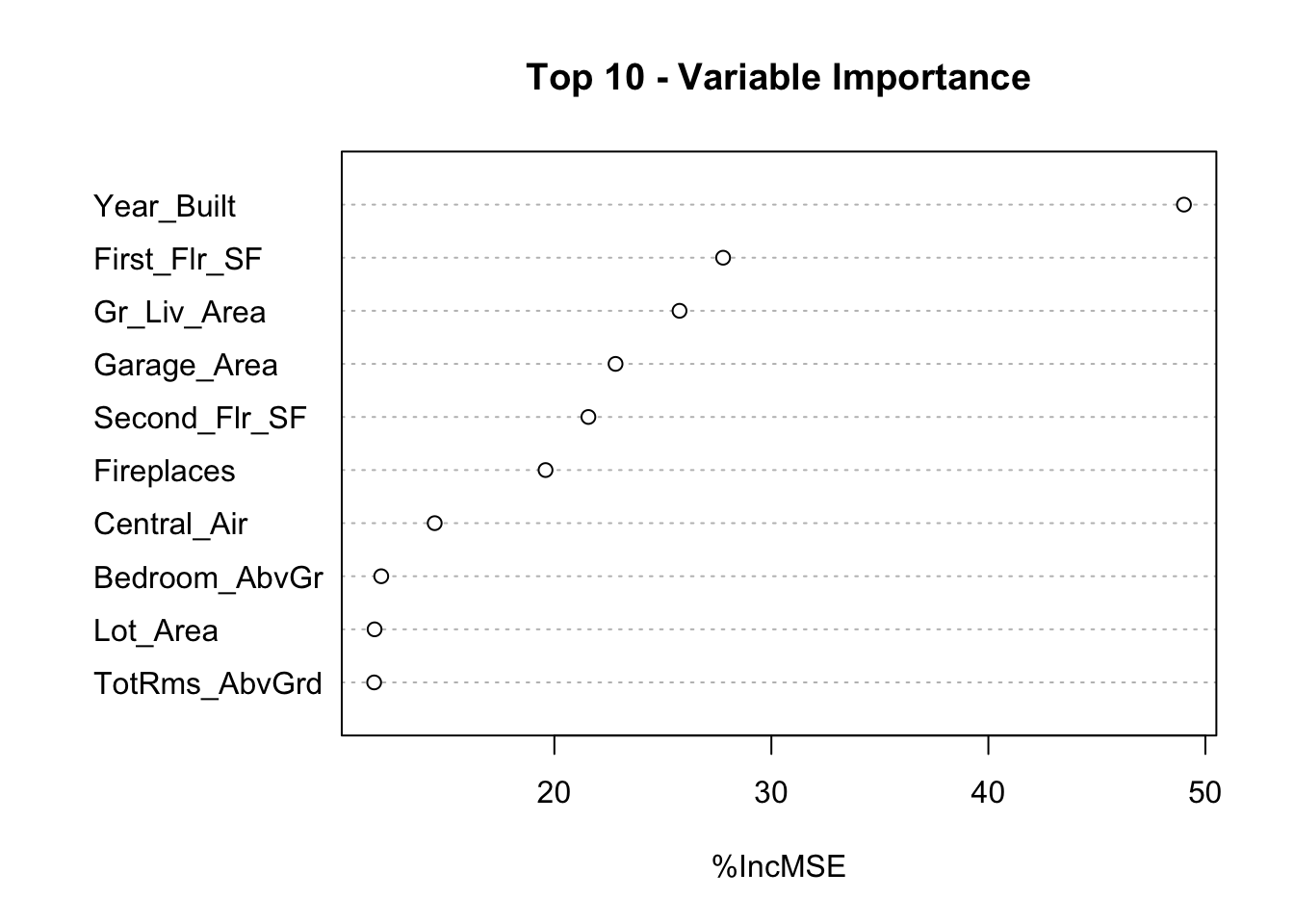
We can use the varImpPlot function to plot the variables by importance in the random forest. The sort = TRUE option sorts the variables from best to worst, while the n.var option controls how many variables are shown. Every variable is in the random forest to some degree. The importance function will list the variables’ actual values of importance instead of just plotting them.
Code
library(randomForest)set.seed(12345)rf.ames <-randomForest(Sale_Price ~ ., data = training.df, ntree =250, importance =TRUE)varImpPlot(rf.ames,sort =TRUE,n.var =10,main ="Top 10 - Variable Importance", type =1)
The plot above shows the percentage increase in MSE when the variable is “excluded” from the model. In other words, how much worse is the model when that variable’s impact is no longer there. The variable isn’t actually removed from the modeling process, but the values are permuted (randomly shuffled around) to remove the impact of that variable. According to permutation importance, Year-Built is by far the most important variable.
However, we want to calculate this for any model, not just our random forest. To do this we will need the iml package. Let’s build a linear regression model using the lm function. Similar to a lot of modeling functions in R, we have a formula input as well as a data option to enter the training dataset. We can use the summary function to look at the variables that are significant in the model.
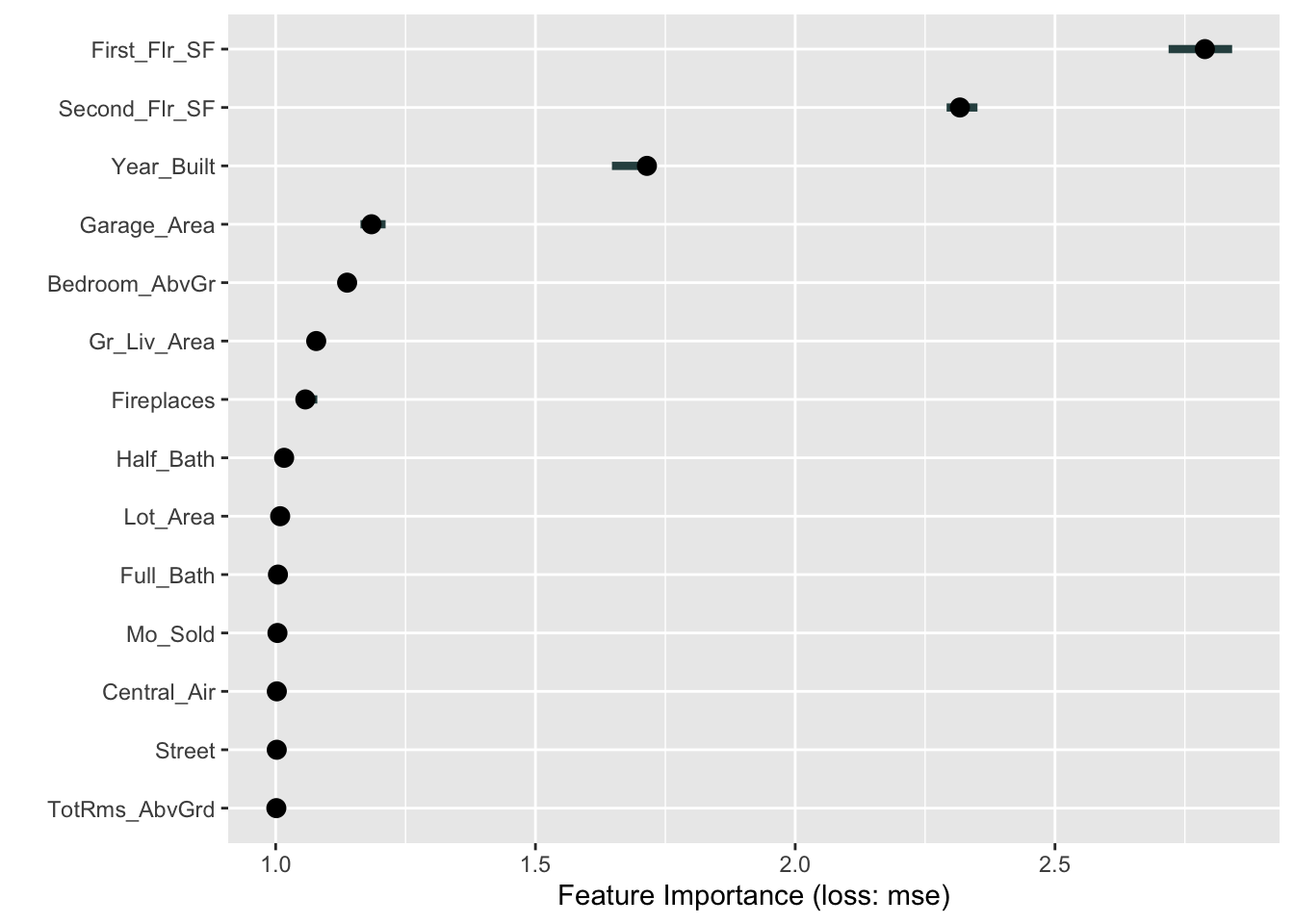
We use the Predictor$new functionality of the iml package to build out the permutation importance of this linear regression. We use the lm model object as an input as well as the training dataset without the target variable, here column 1, in the data option. The y = option is where we specify the target variable, Sale_Price. The type = 'response' option tells R we want the predictions to be in the same scale as the continuous target variable. Lastly, we use the Feature$Imp function on this prediction object. We specify the loss function we want which is just how we evaluate our variables. Here we want our variables evaluated with mean squared error, loss = 'mse'. The plot function just plots the results.
Code
library(iml)lm.ames <-lm(Sale_Price ~ ., data = training)summary(lm.ames)
linear_pred <- Predictor$new(lm.ames, data = training[,-1], y = training$Sale_Price, type ="response")plot(FeatureImp$new(linear_pred, loss ="mse"))
From the output above we have the summary of the original linear regression model as well as the permutation importance plot. Notice how there are some slight differences between them. The Year_Built and Garage_Area variables have the lowest p-values. However, in the permutation importance calculation, these are the 3rd and 4th most important variables behind first and second floor square footage. Although we see some slight deviations, the techniques mostly agree that size of home, year built, size of garage, and number of bedrooms are very important to determining the price of the home.
Before calculating the permutation importance, we need to build our random forest model. We will use the RandomForestRegressor function from the sklearn.ensemble package. Similar to other Python functions we have used, we need the training predictor variables in one object and the target variable in another used in the fit function as X = and y = respectively. The option to define how many decision trees are in the ensemble is n_estimators. We optimized this value earlier to 500. We also have the max_features option, also called \(mtry\), which was optimized to 7.
In a Jupyter environment, please rerun this cell to show the HTML representation or trust the notebook. On GitHub, the HTML representation is unable to render, please try loading this page with nbviewer.org.
To get our permutation importance calculation we will use the skexplain package from scikit-learn. We will use the ExplainToolkit function where we input our model (along with a name, ('Random Forest, rf_ames')) as well as our predictor variables and target variable in the usual X = and y= options from scikit-learn. Next, we use the permutation_importance function on the above ExplainToolkit object. We want to see all 14 variables in the calculation (n_vars = 14). We specify the loss function we want which is just how we evaluate our variables. Here we want our variables evaluated with mean squared error, evaluation_fn = 'mse'. We want 5 permutations of each variable (n_permute = 5) and set a random seed to make our results repeatable.
We take the results from that permutation_importance function and put them into the plot_importance function on the original ExplainToolkit object. We define the panels to see as a backward_singlepass through the permutation calculation on the model we named in the ExplainerToolkit function. The backward single-pass approach was described above. This is great for variables that have little dependence with each other. For highly correlated data, we can use the multi-pass approach which calculates permutation importance while other variables also remain permuted. We stillw ant to plot all 14 of our variables and just change the label on the x-axis.
Code
import skexplainexplainer = skexplain.ExplainToolkit(('Random Forest', rf_ames), X = X_train, y = y_train)results = explainer.permutation_importance(n_vars =14, evaluation_fn='mse', n_permute =5, random_seed =12345)
The plot above shows the percentage increase in MSE when the variable is “excluded” from the model. In other words, how much worse is the model when that variable’s impact is no longer there. The variable isn’t actually removed from the modeling process, but the values are permuted (randomly shuffled around) to remove the impact of that variable. According to permutation importance, Year-Built is the most important variable.
However, we want to calculate this for any model, not just our random forest. Since scikit-learn has many different models it can calculate, this becomes easy to do. We will use the LinearRegression function from the linear_model package of scikit-learn. Similar to many other models in Python, we will input the predictor variables and the target variable into the X = and y = options of the fit function on the linear regression object. From there, the rest of the permutation importance calculation code is the same as with the random forest output above.
Code
from sklearn import linear_modellm_ames = linear_model.LinearRegression()lm_ames.fit(X_train, y_train)
LinearRegression()
In a Jupyter environment, please rerun this cell to show the HTML representation or trust the notebook. On GitHub, the HTML representation is unable to render, please try loading this page with nbviewer.org.
LinearRegression()
Code
explainer = skexplain.ExplainToolkit(('Linear Regression', lm_ames), X = X_train, y = y_train)results = explainer.permutation_importance(n_vars =14, evaluation_fn='mse', n_permute =5, random_seed =12345)
According to the linear regression, the variables of most importance is slightly different than the random forest model. The linear regression has the first and second floor square footage as the most important followed by Year_Built and Garage_Area. Although we see some slight deviations, the techniques mostly agree that size of home, year built, and the size of garage are very important to determining the price of the home.
Individual Conditional Expectation (ICE)
General Idea
“Let me show you how the predictions for each observation change if we vary the feature of interest.”
The individual conditional expectation (ICE) is a local interpreter that visualizes the dependence of an individual prediction on a given predictor variable. It fixes all the other variables for a single observation while changing the variable of interest and then plots the results to visualize the predictions vs the predictor variable.
Let’s look at this concept visually. First, we select both a variable of interest and a single observation. We will still look at our Garage_Area variable, but only for the first observation:
Next, we will replicate this single observation over and over into a new dataset while holding all the other variables constant and not allowing their values to change. We will then fill in values for the variable of interest across the entire range of the variable:
Lastly, we will use the model to predict the target variable in each of these simulated observations:
This will give us an idea of how that single observation is impacted by that variable we are interested in. We will then repeat this calculation for each of the observations in our dataset (or a large sample of them).
We will continue to use the same random forest model from above. We still use the Predictor$new functionality of the iml package to build out the ICE for the random forest. We use the random forest model object as an input as well as the training dataset without the target variable, here column 1, in the data option. The y = option is where we specify the target variable, Sale_Price. The type = 'response' option tells R we want the predictions to be in the same scale as the continuous target variable.
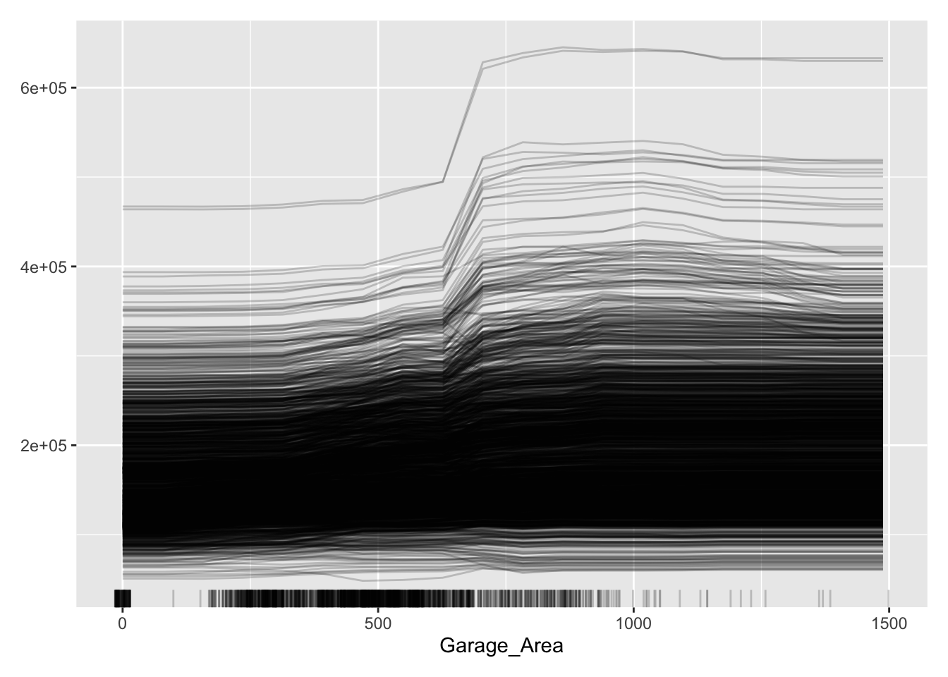
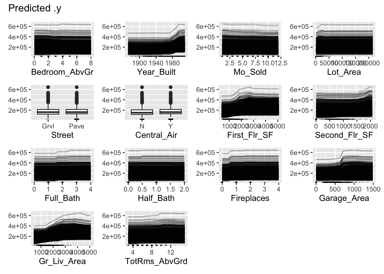
Lastly, we use the FeatureEffects$new function on this prediction object. We specify the method we want to use for our interpreter which is method = 'ice'. The plot element just plots the results. To specify a specific variable we can input that variable name into the plot function. Otherwise, it will produce ICE plots for all of the variables.
Code
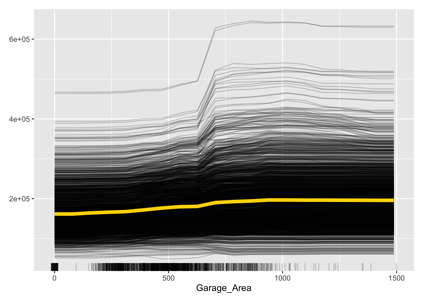
library(patchwork)set.seed(12345)forest_pred <- Predictor$new(rf.ames, data = training[,-1], y = training$Sale_Price, type ="response")ice_plot <- FeatureEffects$new(forest_pred, method ="ice")ice_plot$plot(c("Garage_Area"))
Code
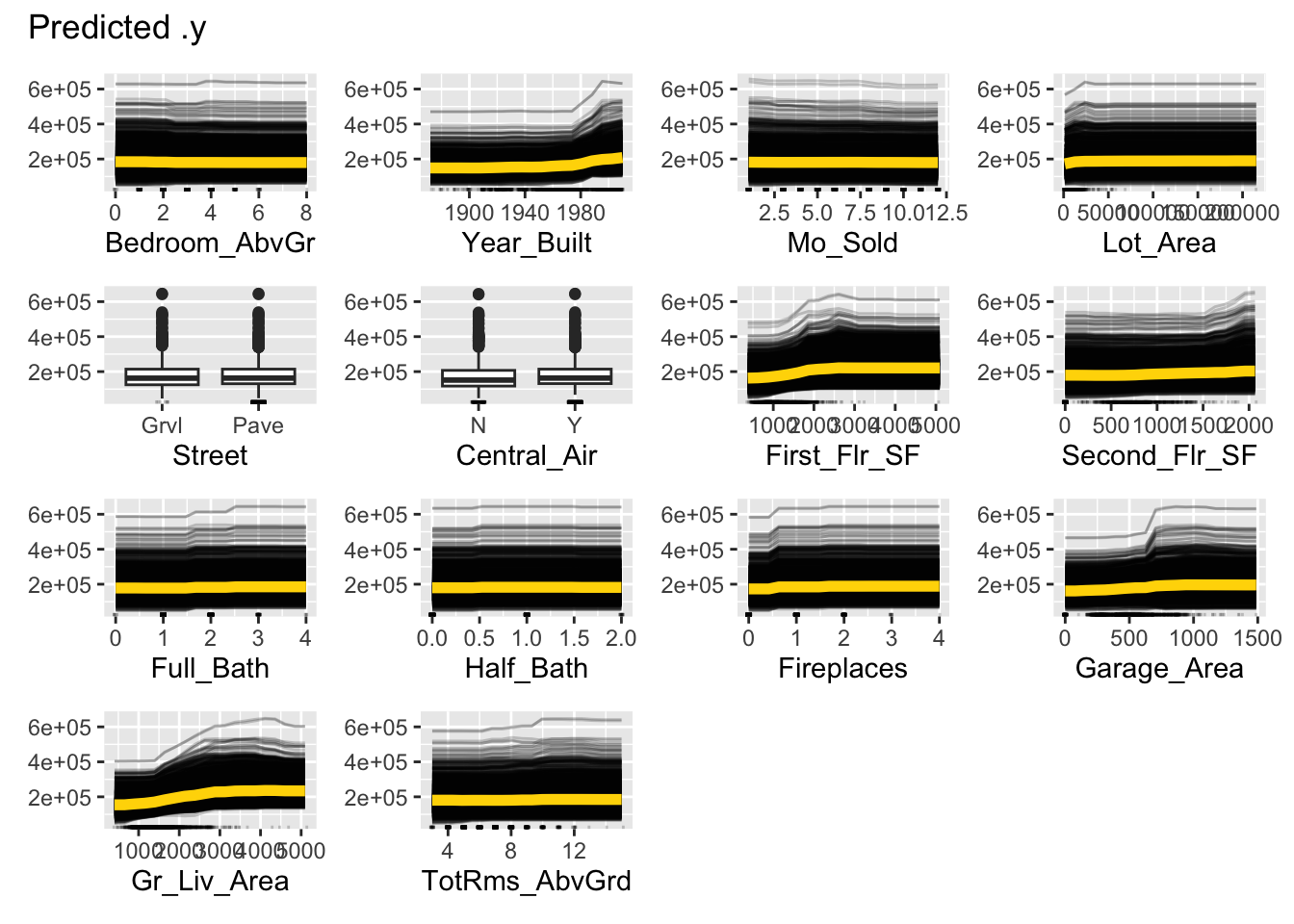
ice_plot$plot()
Let’s take a look at the results above. These plots have the possibility of overwhelming people the first time they see them. In reality, these plots don’t serve too much value when you plot all of the lines on the same plot. As we can see with the Garage_Area plot, there are different patterns going on for different observations. ICE is a local method which is best used to just explore the plot of a single observation, or just examine the predictions of a single observation.
We will continue to use the same random forest model from above. To get our ICE calculation we will use the skexplain package from scikit-learn. We will use the ExplainToolkit function where we input our model (along with a name, ('Random Forest, rf_ames')) as well as our predictor variables and target variable in the usual X = and y= options from scikit-learn.
Next, we use the ale function on the above ExplainToolkit object. We want to see the calculation for a specific variable, Garage_Area. Next, we also use the ice function on the ExplainToolkit object with the same feature of interest. Lastly, we use the plot_ale function on the original ExplainToolkit object with the ale and ice objects serving as inputs to the ale and ice_curves options respectively. Again, we have to specify the model name, here in the estimator_names option. After a couple of label and figure options for viewing, we have our ICE plot.
Code
explainer = skexplain.ExplainToolkit(('Random Forest', rf_ames), X = X_train, y = y_train)ale = explainer.ale(features ='Garage_Area', n_bootstrap =2, n_bins=20)
ALE Numerical Features:   0%|          | 0/1 [00:00<?, ?it/s]
ALE Numerical Features: 100%|##########| 1/1 [00:00<00:00, 10.40it/s]
Let’s take a look at the results above. These plots have the possibility of overwhelming people the first time they see them. In reality, these plots don’t serve too much value when you plot all of the lines on the same plot. As we can see with the Garage_Area plot, there are different patterns going on for different observations. There is also a histogram of the Garage_Area variable hidden in the background as well. ICE is a local method which is best used to just explore the plot of a single observation, or just examine the predictions of a single observation.
One of the biggest disadvantages of ICE is the impact of multicollinearity. If the variable of interest is correlated with other predictor variables, some of the simulated data may be invalid. Let’s take a look at Garage_Area across values of first floor square footage:
Since we are fixing first floor square footage for a single observation and then simulating all of the possible values of Garage_Area, we could get some nonsensical values. As we can see by the horizontal dots above, a home with 2400 square feet on the first floor would reasonably have values of Garage_Area in between 500 and 1300 square feet. However, we are simulating these homes all the way down to no garage and up to values of 1500 square feet. Therefore, we must be careful when interpreting ICE predictions for a single observation as some of the predictions are extrapolating outside of the reasonable range of values.
Partial Dependence
General Idea
“Let me show you what the model predicts on average when each observation has the value k for that feature, regardless if that value makes sense.”
A partial dependence plot (PDP) is a global interpreter that attempts to show the marginal effect of predictor variables on the target variable. Marginal effects are averaged effects over all possible values of a single variable. Essentially, the PDP is the average of the ICE plots discussed in the section above.
Let’s look at this concept visually. First, choose a variable of interest. We will look at Garage_Area. Next, we will replicate the entire dataset while holding all variables constant except for the variable of interest:
Next, we will fill the variable of interest column in each dataset with one of the possible values (determined by the range of the data) of the predictor variable of interest:
We will use our model to generate predictions across all of the rows of each of the datasets. The predictions from each dataset will be averaged together and they will correspond to a particular value of the predictor variable of interest. That means we will have a dataset and prediction for each of the values in the range of Garage_Area which is 0 to 1488:
This will give us an idea of how that are target variable is impacted on average by that variable we are interested in. The visual of this will hopefully show the potentially complex relationship between that predictor variable and the target variable.
We will continue to use the same random forest model from above. We still use the Predictor$new functionality of the iml package to build out the PDP for the random forest. We will not repeat all the code for the Predictor$new function as it is listed above.
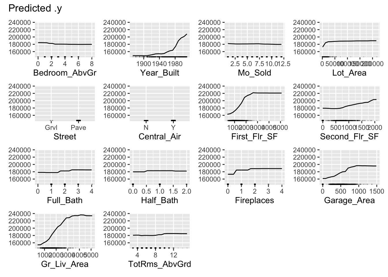
We use the FeatureEffects$new function on this prediction object from the Predictor$new function. We specify the method we want to use for our interpreter which is method = 'pdp'. The plot element just plots the results. To specify a specific variable we can input that variable name into the plot function. Otherwise, it will produce PDP plots for all of the variables.
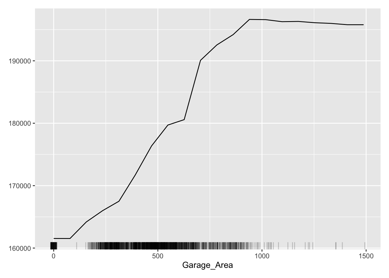
This nonlinear and complex relationship between Garage_Area and Sale_Price is similar to the plot we saw earlier with the GAMs, random forests, and XGBoost model sections. This shouldn’t be too surprising. All of these algorithms are trying to relate these two variables together, just in different ways.
If we wanted to see the PDP plotted on top of the ICE plots to get a better sense of what we are averaging to get the PDP line we can just switch the method = 'pdp' option to method = 'pdp+ice'.
We will continue to use the same random forest model from above. To get our PDP calculation we will use the skexplain package from scikit-learn and the ExplainToolkit function. We will not repeat all the code for the ExplainToolkit function as it is listed above.
To get the PDP we use the pdp function on the above ExplainToolkit object. We want to see the calculation for a specific variable, Garage_Area. However, we are not limited to just viewing one at a time so we put two additional variables to see their PDP values as well. Lastly, we use the plot_pdp function on the original ExplainToolkit object with the pd object serving as input to the pd option.
This nonlinear and complex relationship between Garage_Area and Sale_Price is similar to the plot we saw earlier with the GAMs, random forests, and XGBoost model sections. This shouldn’t be too surprising. All of these algorithms are trying to relate these two variables together, just in different ways.
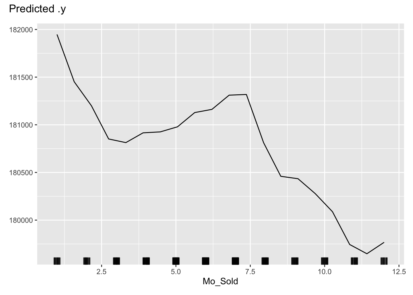
One thing you should always be careful of when plotting our PDPs is the scale of the data. Most plotting functions across softwares will adjust the scale of the plot for you. This is not always helpful. Take a look at the plot below with the variable describing the month in which is the house is sold.
Code
pd_plot$plot(c("Mo_Sold"))
This looks like there is a big change across different months of the year. However, if we focus on the y-axis, we see that these changes all occur within a couple of thousand dollars.
Accumulated Local Effects (ALE)
General Idea
“Let me show how the model predictions change when I change the variables of interest to values within a small interval around their current values.”
Partial dependence plots are an average of ICE plots which we previously discussed have problems with multicollinearity. If the variable of interest is correlated with other predictor variables, some of the simulated data may be invalid. Let’s take a look at Garage_Area across values of first floor square footage:
Since we are fixing first floor square footage for a single observation and then simulating all of the possible values of Garage_Area, we could get some nonsensical values. As we can see by the horizontal dots above, a home with 2400 square feet on the first floor would reasonably have values of Garage_Area in between 500 and 1300 square feet. However, we are simulating these homes all the way down to no garage and up to values of 1500 square feet.
Instead of looking at all values like ICE, and therefore PDP, the accumulated local effects (ALE) global interpreter uses only reasonably contrived data to get a clearer picture of the relationship between a variable of interest and the target variable. By default, ALE uses quantiles of your data to define this reasonable range of values. For observations in each interval, we determine how much their prediction would change if we replace the feature of interest with the upper and lower bounds of the interval, while keeping all other variables constant. Let’s look at his visually:
With the ALE we will do this calculation for all of the observations in the interval. This allows us to understand how the predictions are changing within a reasonable window around the data values for the predictor variable.
Let’s see how to do this in each of our softwares!
We will continue to use the same random forest model from above. We still use the Predictor$new functionality of the iml package to build out the ALE for the random forest. We will not repeat all the code for the Predictor$new function as it is listed above.
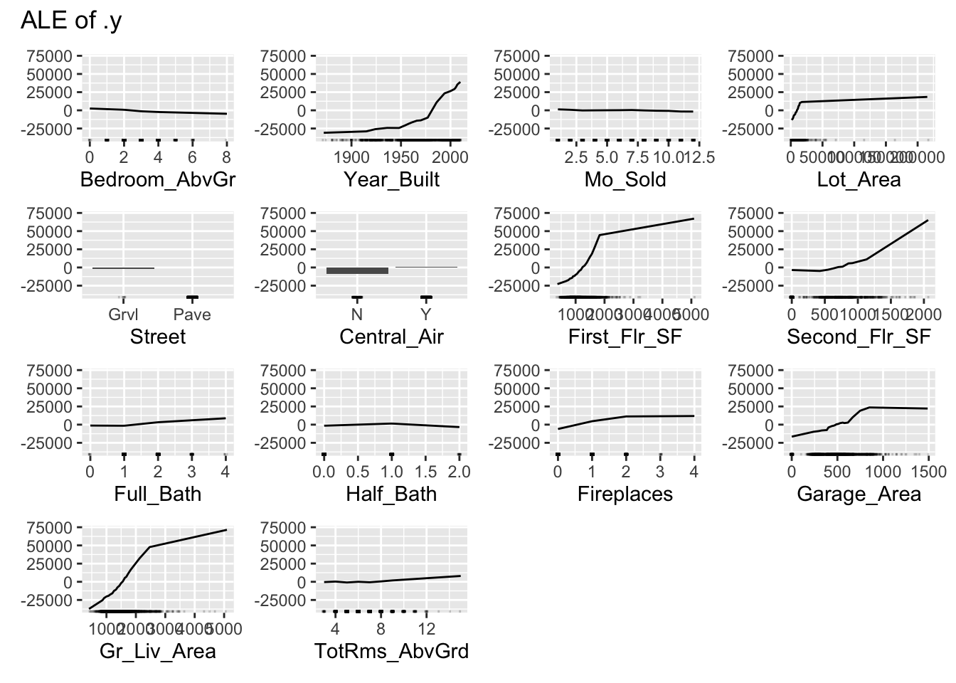
We use the FeatureEffects$new function on this prediction object from the Predictor$new function. We specify the method we want to use for our interpreter which is method = 'ale'. The plot element just plots the results. To specify a specific variable we can input that variable name into the plot function. Otherwise, it will produce ALE plots for all of the variables.
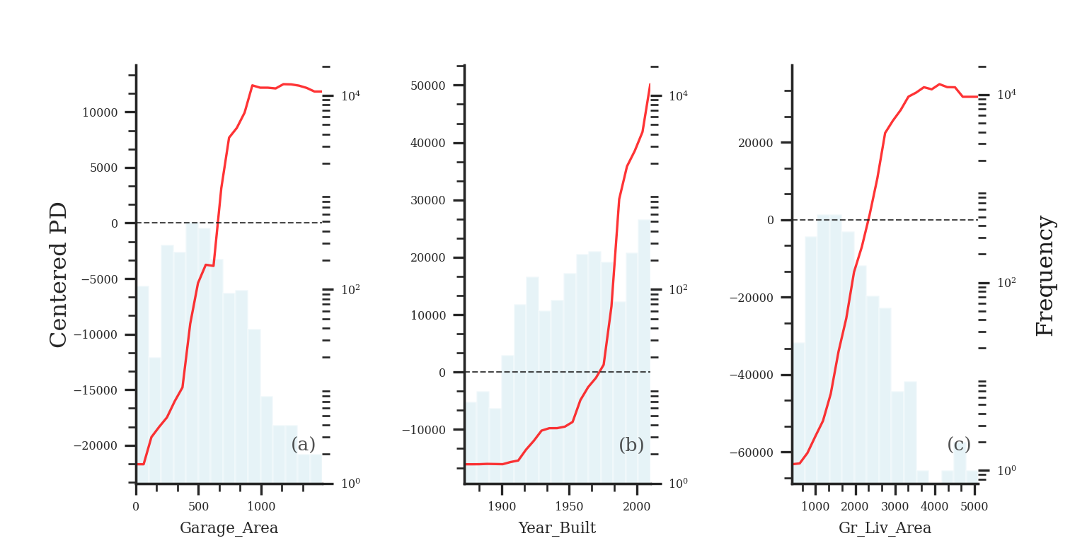
The ALE curve that is provided is a centered calculation. This means that the ALE describes the main effect of the predictor variable compared to the data’s average prediction. For example, in the plot above for Garage_Area, the value of 700 square feet for Garage_Area corresponds to a value of $10,000 in ALE. This means that when Garage_Area is 700 square feet, the prediction for our sale price is $10,000 higher than the average prediction in our model.
Another interesting point to observe on an ALE plot is the spot where the values go from negative to positive. Again, using the Garage_Area plot above, we see that around 500 square feet of Garage_Area the effect on the prediction of sale price of the home changes from negative to positive. Therefore, homes with values smaller than 500 square feet lead to a below average prediction as compared to homes above 500 square feet have an above average prediction.
We will continue to use the same random forest model from above. To get our ALE calculation we will use the skexplain package from scikit-learn and the ExplainToolkit function. We will not repeat all the code for the ExplainToolkit function as it is listed above.
To get the ALE we use the ale function on the above ExplainToolkit object. We want to see the calculation for a specific variable, Garage_Area. However, we are not limited to just viewing one at a time so we put two additional variables to see their ALE values as well. Lastly, we use the plot_ale function on the original ExplainToolkit object with the ale object serving as input to the ale option.
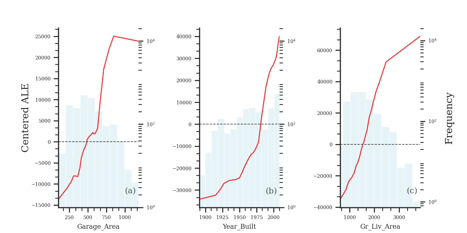
The ALE curve that is provided is a centered calculation. This means that the ALE describes the main effect of the predictor variable compared to the data’s average prediction. For example, in the plot above for Garage_Area, the value of 700 square feet for Garage_Area corresponds to a value of $10,000 in ALE. This means that when Garage_Area is 700 square feet, the prediction for our sale price is $10,000 higher than the average prediction in our model.
Another interesting point to observe on an ALE plot is the spot where the values go from negative to positive. Again, using the Garage_Area plot above, we see that around 500 square feet of Garage_Area the effect on the prediction of sale price of the home changes from negative to positive. Therefore, homes with values smaller than 500 square feet lead to a below average prediction as compared to homes above 500 square feet have an above average prediction.
Local Interpretable Model-Agnostic Explanations (LIME)
General Idea
“Let me show you a linear model that could explain the exact orientation of the predictive model at a specific point.”
The best way to understand the local interpreter LIME is through a visual. Imagine that you had a nonlinear relationship between a target and a predictor variable. Now imagine you zoom in really close to a specific point of interest as in the figure below:
That zoomed in area around the point of interest looks like an approximately straight line. We know that we can model (and interpret) straight lines with linear regression. This will help us understand the effects or impact of that variable of interest around our point of interest. Of course, we can expand this linear regression to include all of the variables and not just one.
Here are the basic steps of what LIME is doing:
Randomly generate values (usually, normally distributed) for each variable in the model.
Weight more heavily the fake observations that are near the real observation of interest.
Build a weighted linear regression model based on fake observations and the observation (row in the dataset) of interest.
“Interpret” the coefficients of variables and their “impact” from the linear regression model.
LIME is not actually limited to linear regression and we could use any interpretable model (decision tree for example). One of the biggest choices we have in LIME is the number of variables we use in the local linear regression model. Typically, we don’t use all of the variables in a local model like LIME as we are trying to focus on the main driving factors. However, the definition of “near the points of interest” is a very big and unsolved problem in the world of LIME.
Let’s see how to do this in each of our softwares!
We will continue to use the same random forest model from above. We still use the Predictor$new functionality of the iml package to build out the LIME for the random forest. We will not repeat all the code for the Predictor$new function as it is listed above.
For LIME we will use the LocalModel$new function. We will still use the same Predictor$new object from above in this function. The only other input is the specific observation that we want to “interpret,” which is observation number 1328 in the example below. The k = 5 option tells the LIME process to use only use 5 variables for the local model. We can look at both a plot of the results (using the plot function) or just the LIME results directly by looking at the results element of the LocalModel$new object.
Code
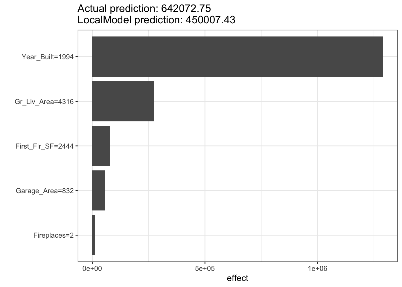
point <-1328lime.explain <- LocalModel$new(forest_pred, x.interest = training[point,-1], k =5)plot(lime.explain) +theme_bw()
Let’s first examine the plot. The bars in the plot represent the “effect” of the variables. This effect is the slope of the linear regression for that variable multiplied by the values of the variable itself, essentially \(\beta_i x_i\). The tabular results can help us see this a little more. For example, the Year_Built variable has a slope coefficient for the local regression of 647.22. This house specifically was built in 1994. That means the “effect” of that variable is 1,290,551.21. The biggest takeaways from the plot above is the variables that have the most “effect.” Notice that the Fireplaces variable has the biggest slope for the local regression, but since it take a value of 2, the “effect” for this observation is still smaller than other variables.
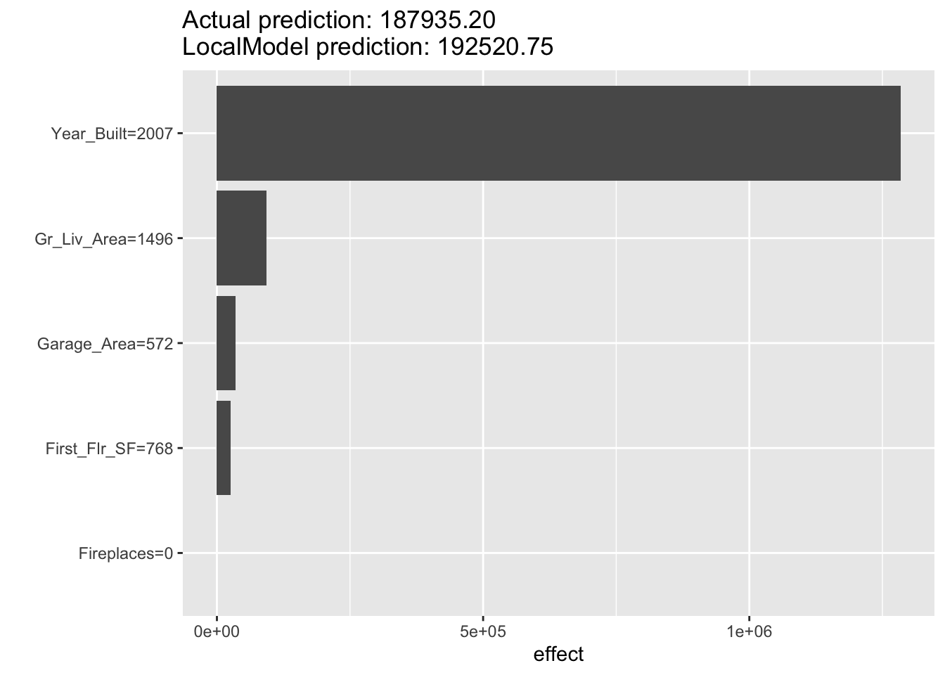
Let’s take a look at how this might change for another observation. Instead of observation 1328, let’s explore observation 1000 with the same code.
Code
point <-1000lime.explain <- LocalModel$new(forest_pred, x.interest = training[point,-1], k =5)plot(lime.explain)
From the above output we can see that the variable Year_Built still has the greatest effect on our prediction, but the order and magnitude of the variables is different because this is a different, local linear regression.
For LIME we are going to use a different package in Python, namely the lime package. From the lime package we will import the lime_tabular package. From this set of packages we will use the LimeTabularExplainer function which has an array of inputs we need to fill in. The first input is the values from your training dataset. Since our dataset is a data frame, we will use the .values function to extract just the values. We then need to give the function the names of the training dataset variables in the feature_names option using the columns function on our training data frame. The class_names option is where we specify the name of the target variable. Next, we need to give the function the names of the categorical variables with the categorical_features option. Lastly, we need to specify the mode = 'regression' option so the model knows the input is a regression model and not a classification model.
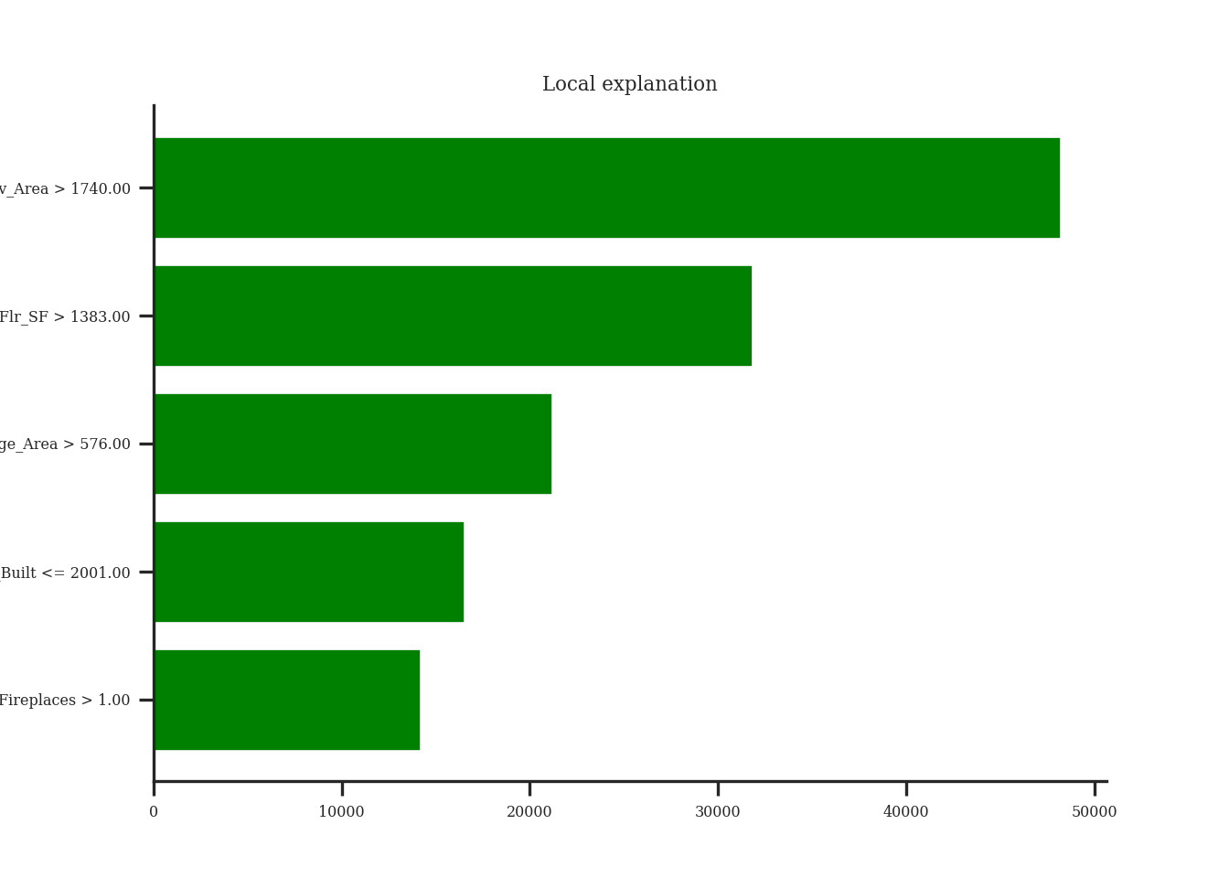
Now that we have our LimeTabularExplainer object defined, we can use the explain_instance function on this object. The inputs to the explain_instance function are the specific observation you are interested in, here observation 1328, the predictions from our random forest model (using the predict function), and the number of variables we want in the local regression. The results from the LIME model can be seen in either a list using the as_list() function or in a plot using the as_pyplot_figure() option.
Let’s first examine the plot. The bars in the plot represent the “effect” of the variables. This effect is the slope of the linear regression for that variable multiplied by the values of the variable itself, essentially \(\beta_i x_i\). Since all of these “effects” are from a linear regression, we can add them together to get the predicted value from the local linear regression. This truly allows us to see how the prediction is broken down by each variable. We can see this even more with the list output. We can see the intercept from the linear regression along with the “effects” of each of the variables. These added together sum up to the predicted value listed in the output as well.
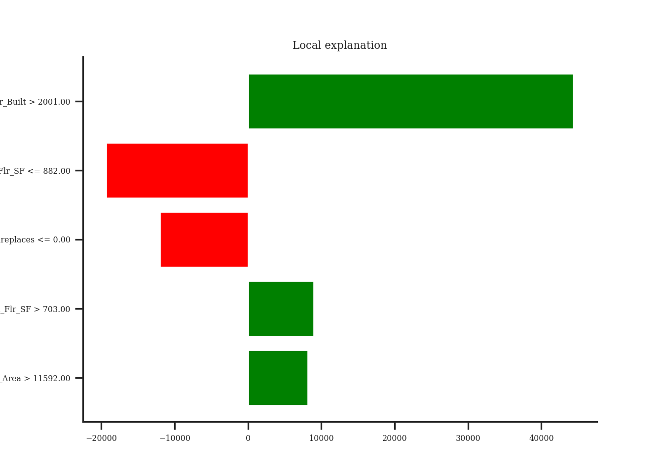
The biggest takeaways from the plot above is the variables that have the most “effect” locally on that observation. This could change for each observation. Instead of observation 1328, let’s explore observation 1000 with the same code.
From the above output we can see that the variable Year_Built still has the greatest effect on our prediction, but the order and magnitude of the variables is different because this is a different, local linear regression. We can even see with this observation that some of the variables had a negative impact on our predicted sale price. For example, the smaller first floor square footage actually decreased our sale price prediction locally by almost $18,900.
Shapley Values
General Idea
“Let me show you the value the \(j^{th}\) feature contributed to the prediction of this particular observation compared to the average prediction of the whole dataset.”
As mentioned above, the general idea for the Shapley value local interpreter is to measure the “effect” of a specific variable on the difference in the prediction of a specific point compared to the overall prediction. This is best seen through an example. In Python, the predicted sale price of observation 1328 is $672,791.28 from our random forest. The average, predicted sale price of homes from the random forest is $180,628.03. Let’s now look at the Shapley values for observation 1328:
If we were to take all of the pieces you see above and sum them together, \(13,754.21 + 93,854.94 + \cdots + 6.14 = 492,163.25\). This is the exact difference between our predicted value of $672,791.28 and the overall prediction of $180,628.03. This means we can directly see how each variable impacts our specific prediction of observation 1328 in terms of the predicted sale price of the home.
This sounds great, but how does it work in the background? It goes back to the mathematical idea of game theory. Shapley (1953) assigned a payout values for players depending on their contribution to the total payout across a coalition (think team). In other words, imagine you have a team of basketball players playing in a local tournament. You all win some money in the local tournament. How do you split the winnings? Evenly? Maybe. Or you could split the winnings based on contribution to the team. The star player gets the most, followed by the second best player, and so on all the way down the team. That is the idea of a Shapley value in game theory.
The Shapley value in machine learning is the average marginal contribution of a variable / feature (teammate) across all possible coalitions of variables (possible combinations of teammates). For this we would need to compute the average change in the prediction that a set of variables experiences when the variable of interest is added to the coalition. This computation is done across all observations and across all possible combinations of variables. This calculation can be very time consuming to do with large numbers of variables. There has been a tremendous amount of research in machine learning on how to accomplish this calculation much quicker, such as sampling, subsets of variables, etc.
The creators of Shapley values in machine learning tout four factors for Shapley values that, they argue, makes it one of the best local interpreters.
Efficiency - variable contributions must sum to the difference of the prediction for the point of interest compared to the average prediction.
Symmetry - contributions of two variables should be the same if they contribute equally to all possible combinations of variables.
Dummy - a variable that does not change the predicted value, for any combination of variables, should have a Shapley value of 0.
Additivity - for a forest of trees, the Shapley value of the forest for a given observation should be the average of the Shapley values for each tree at that given point.
We will continue to use the same random forest model from above. We still use the Predictor$new functionality of the iml package to build out the Shapley values for the random forest. We will not repeat all the code for the Predictor$new function as it is listed above.
We will input the Predictor$new object into the Shapley$new function. The only other option we need to specify is the specific observation we are interested in. Here we will look at observation 1328 like we did with LIME. All we need to input is the training dataset predictor values at that specific point. Lastly, we just call the plot() function on that Shapley$new object to visualize the values.
Code
point <-1328shap <- Shapley$new(forest_pred, x.interest = training[point,-1])shap$plot()
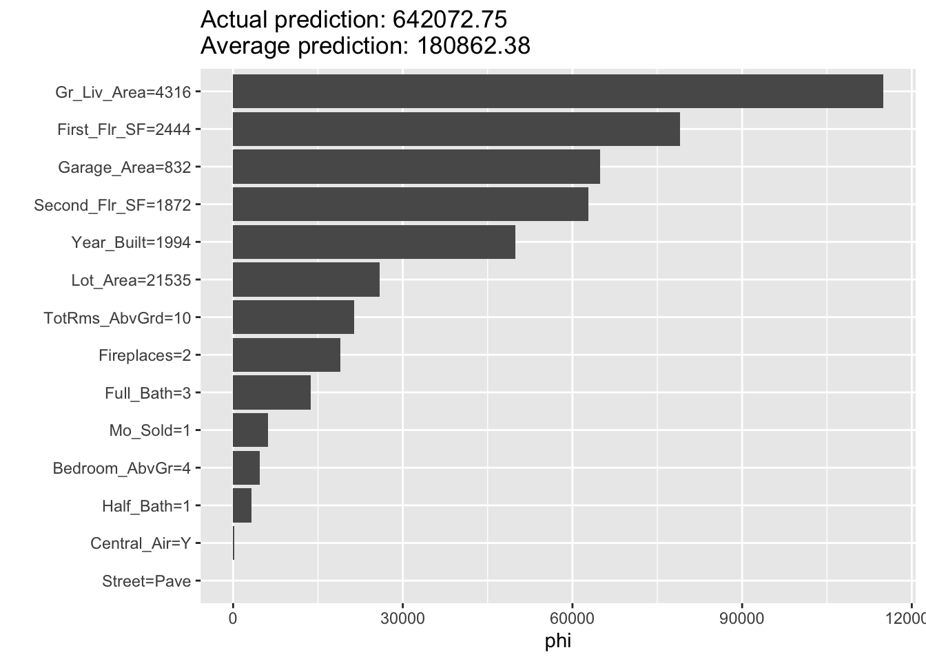
Similar to the Python example worked out above, this plot gives us the overall prediction of sale price across the whole dataset as well as the specific prediction of observation 1328 from our random forest. The bars in the plot represent the impact that a variable has in the difference between that average prediction and the specific prediction of the point. We can see that the Gr_Liv_Area variable has the greatest impact on the difference in prediction.
Let’s take a look at how this might change for another observation. Instead of observation 1328, let’s explore observation 1000 with the same code.
Code
point <-1000shap <- Shapley$new(forest_pred, x.interest = training[point,-1])shap$plot()
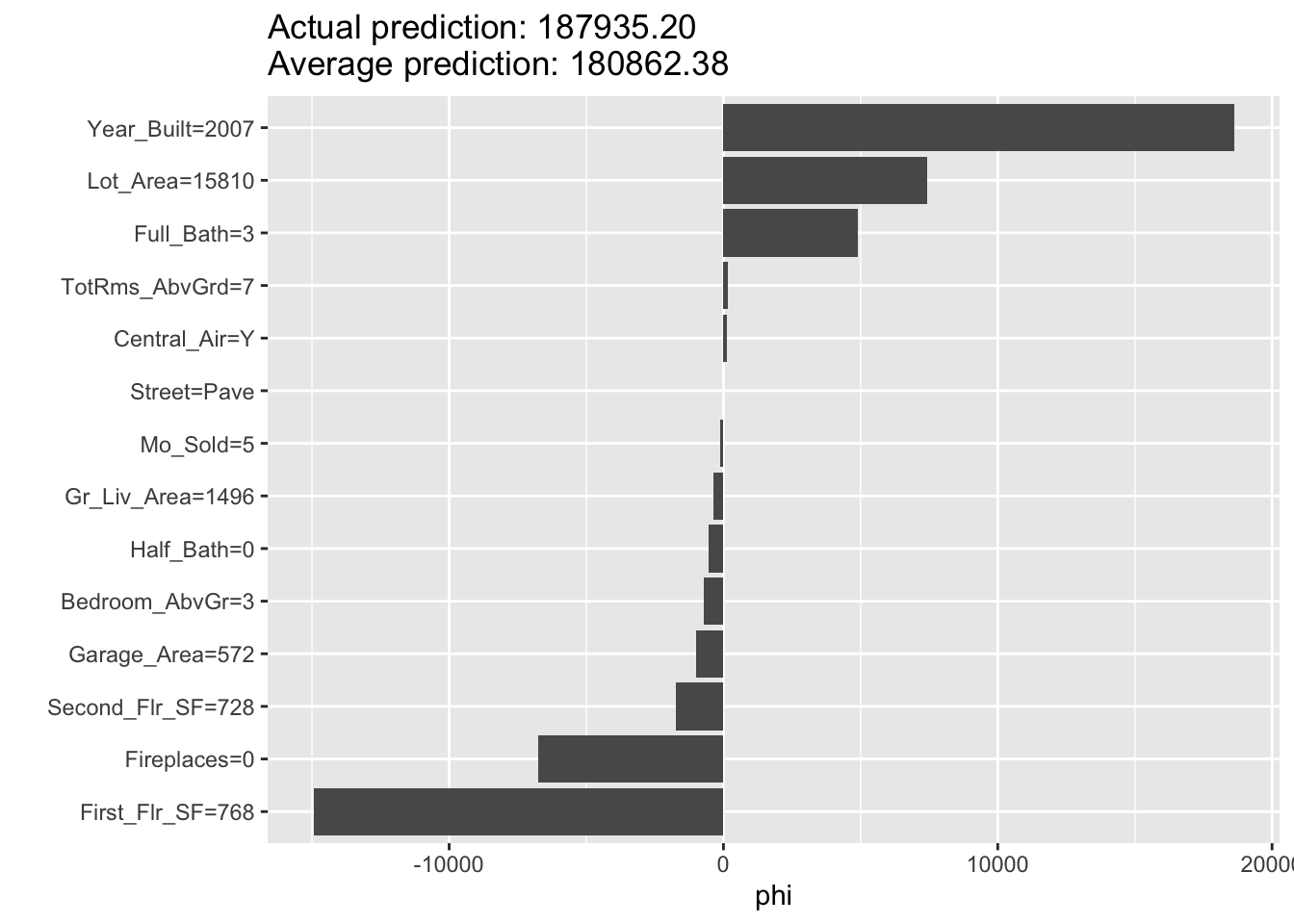
From the above plot we can see drastically different effects for this observation compared to observation 1328. Here, the Year_Built variable has the greatest positive impact on the difference in predicted sales price. However, this observation also has some values that are negatively impacting our prediction. For example, the small first floor square footage appears to have a strong negative impact on our prediction.
For Shapley values we will need to use a different package in Python, the shap package. We are also loading in matplotlib.pyplot for some of the plotting options on the Shapley values. From the shap library we need the Explainer function. The input to this function is the random forest model we have previously built. With this new Explainer object we input the predictor variables from the training dataset to get the Shapley values.
Code
import shapimport matplotlib.pyplot as pltexplainer = shap.Explainer(rf_ames)shap_values = explainer(X_train)
Now that we have the Shapley values we can visualize them in a variety of ways. First, we have a bar plot of the impact of the individual variables on the difference in prediction. For this we just use the shap.plots.bar function on the Shapley values object. Specifically, we are looking at observation 1328. We also use the max_display option to determine how many variables are plotted. By default, this takes a value of 10, but we want to see all of the variables.
Exactly as the original example worked out above, the bars in the plot represent the impact that a variable has in the difference between that average prediction across all houses form the random forest and the specific prediction of observation 1328. We can see that the Gr_Liv_Area variable has the greatest impact on the difference in prediction.
Let’s take a look at how this might change for another observation. Instead of observation 1328, let’s explore observation 1000 with the same code.
Code
shap.plots.bar(shap_values[999], max_display =16)
From the above plot we can see drastically different effects for this observation compared to observation 1328. Here, the Year_Built variable has the greatest positive impact on the difference in predicted sales price. However, this observation also has some values that are negatively impacting our prediction. For example, the small first floor square footage appears to have a strong negative impact on our prediction.
Cautions
There are some things to be cautious about with Shapley values. Some people try to look at the “overall impact” of a variable across all of the observations. One should be very careful with this approach as Shapley values were designed for local interpretations, not necessarily global ones.
For example, in Python we can use the shap.plots.bar function on all of the Shapley values instead of a specific one. This plot will show us the average of the absolute value of all of the Shapley values for a variable.
Code
shap.plots.bar(shap_values, max_display =16)
One potentially valuable piece of information from the plot above is to see that the variable Gr_Liv_Area has the largest average magnitude of impact compared to the other variables. However, this number doesn’t necessarily capture the variability of the impact. We should not assume that all of the impacts are positive (remember, this is an absolute value) or that all of the observations have this specific impact. We saw in our two examples above that some variables have a positive and negative effect on different observations and there are definitely different magnitudes of impact of the same variable on different observations.
Another common plot you will see with Shapley values is the bee swarm plot from the shap.plots.beeswarm function applied to all Shapley values. This tries to show the variability of the impact of each variable across many different observations. Really, the only value form this plot is that notion of variation, but rarely have I noticed clients understanding or needing this plot. One should be hesitant to share this plot with any non-technical audience.
Code
shap.plots.beeswarm(shap_values, max_display =16)
Source Code
---title: "Model Agnostic Interpretability"format: html: code-fold: show code-tools: trueeditor: visual---```{r}#| include: false#| warning: false#| error: false#| message: falselibrary(AmesHousing)ames <-make_ordinal_ames()library(tidyverse)ames <- ames %>%mutate(id =row_number())set.seed(4321)training <- ames %>%sample_frac(0.7)testing <-anti_join(ames, training, by ='id')training <- training %>%select(Sale_Price, Bedroom_AbvGr, Year_Built, Mo_Sold, Lot_Area, Street, Central_Air, First_Flr_SF, Second_Flr_SF, Full_Bath, Half_Bath, Fireplaces, Garage_Area, Gr_Liv_Area, TotRms_AbvGrd)training.df <-as.data.frame(training)``````{python}#| include: false#| warning: false#| error: false#| message: falsetraining = r.trainingtesting = r.testingimport pandas as pdtrain_dummy = pd.get_dummies(training, columns = ['Street', 'Central_Air'])print(train_dummy)y_train = train_dummy['Sale_Price']X_train = train_dummy.loc[:, train_dummy.columns !='Sale_Price']```# Model PerformanceLet's compare all of the models we have built in this slide deck on that test dataset that we haven't used yet.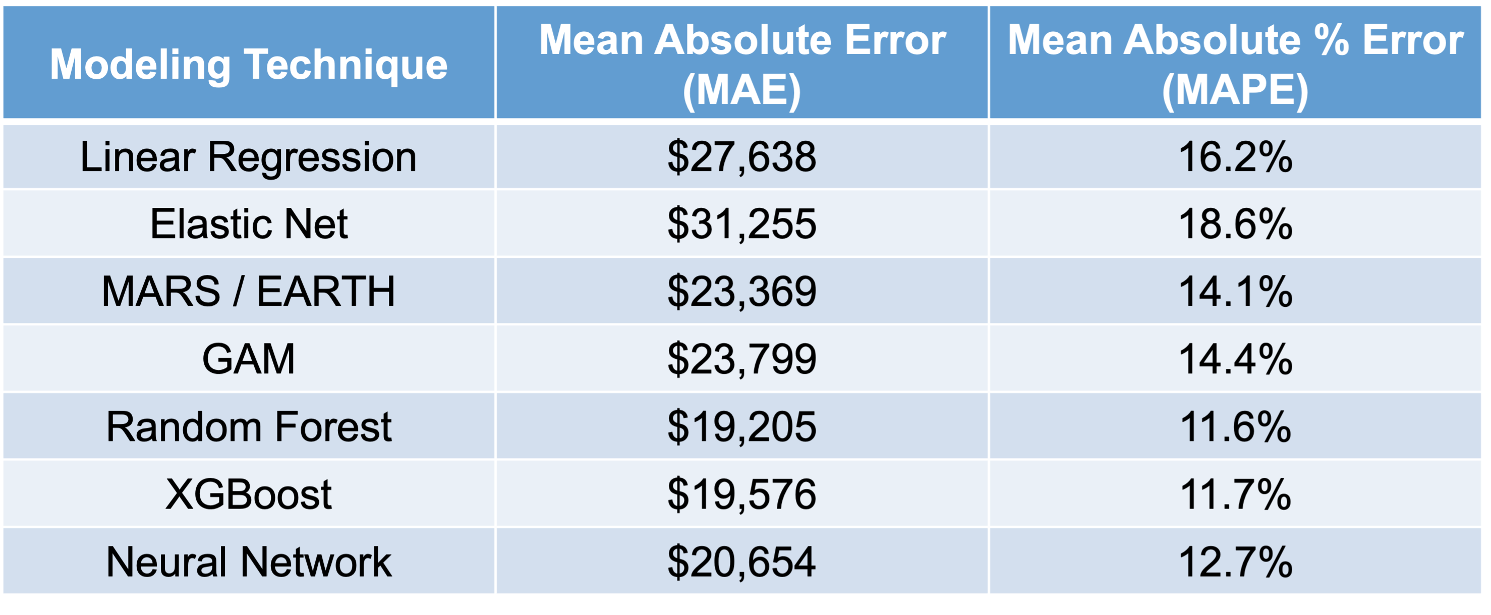{fig-align="center" width="9.71in"}As we can see in the above table, it appears that the most interpretable model - linear regression - is not the one that performs the best for this dataset. It is also not the worst, but the random forest model seems to far outperform it as well as most other models. We will use this random forest in the remaining sections to try and "interpret" our machine learning model.# "Interpretability"Classical, statistical modeling may lend itself easier to interpretation. It is the interpretation that most people are used to with modeling. For example, in linear regression, we have the case of a straight line relationship: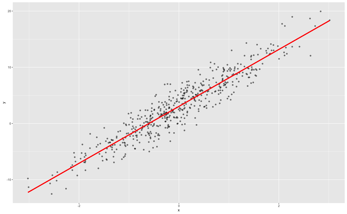{fig-align="center" width="6.49in"}In linear regression, our interpretation is that every single unit increase in *x* (the predictor variable) leads to a $\beta$ unit increase in *y* (the target variable) on average while holding all other variables constant.Decision trees are also considered interpretable models. They have the following step function form: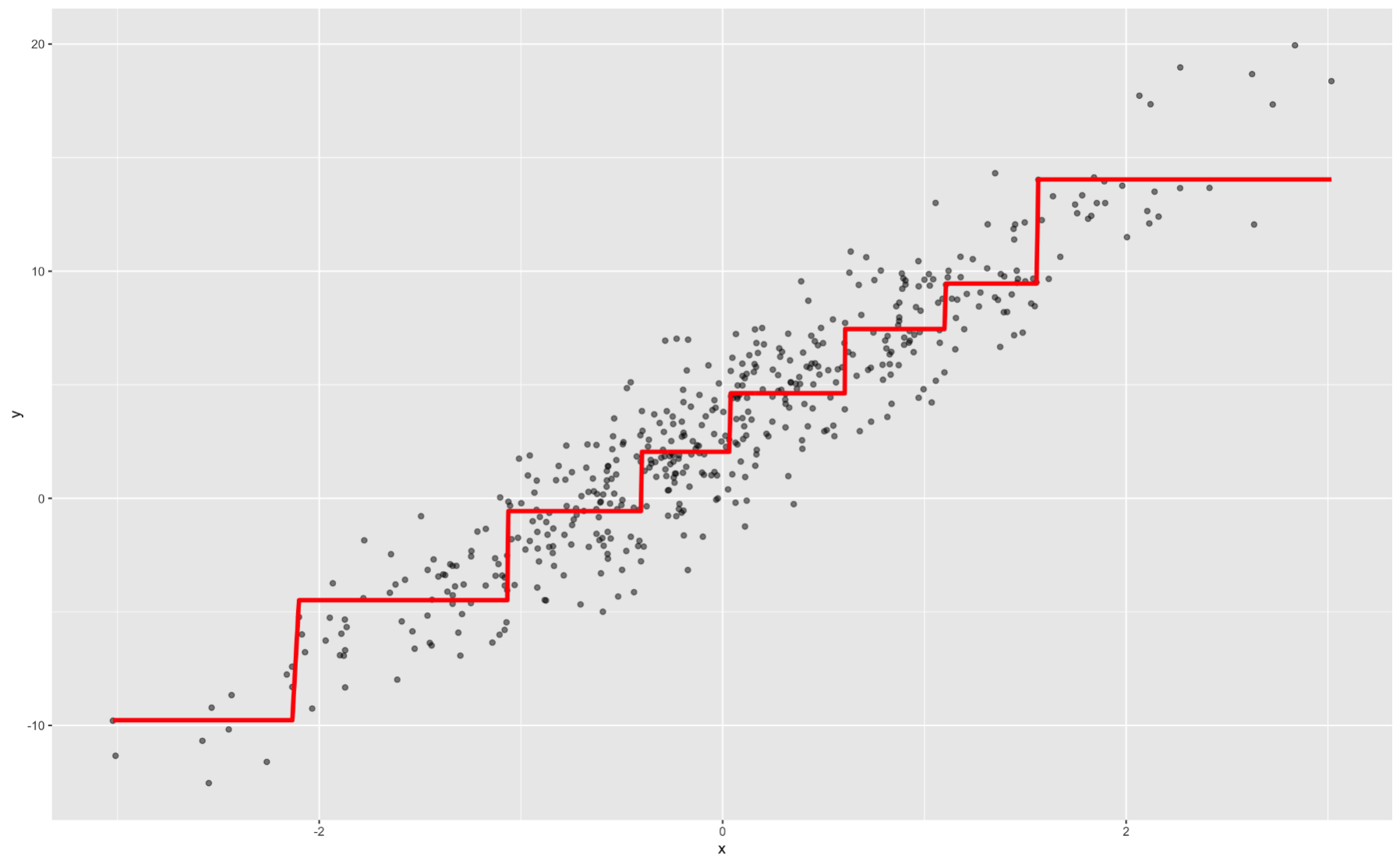{fig-align="center" width="6.49in"}Again, we can interpret ranges of the predictor variable having a specific, estimated relationship with our target.Most machine learning models are not interpretable in these classical approaches. This is mostly because of the nonlinearity of the relationship between the predictor variable and the target variable. Machine learning models are picking up on these more complicated relationships.However, people (especially clients) want to interpret and understand model behavior. There are important questions that drive this need for interpretability:- Why is someone's loan rejected?- Why is this symptom occurring in this patient?- Why is the stock price expected to decrease?Interpretations in machine learning models can be model and/or context specific. Model dependent interpretations are things like variable importance. Variable importance in regression might be different than in tree-based models. A context specific interpretation deals more with the effects of a change in a single variable on a target variable.These important types of interpretations help deal with concepts like fairness / transparency, model robustness / integrity, and legal requirements. With fairness / transparency we need to understand model decisions to improve client and customer trust. These interpretations reveal model behavior on different (and potentially marginalized) groups of people. Model robustness and integrity deals with revealing odd model behavior or overfitting problems where certain variable conclusions don't make intuitive sense. Lastly, there are a number of fields that have legal requirements around models like the Equal Credit Opportunity Act (ECOA), the Fair Credit Reporting Act (FCRA), and more.For machine learning model interpretability, most softwares have collections of two types of interpretations - local and global. These are visualized below: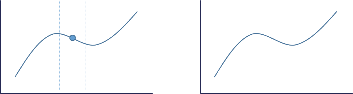{fig-align="center" width="9.32in"}The left plot above is an example of a local interpretation where we can say that *y* decreases as *x* increases **when** *x = 10*. The right hand plot would be more global where we could say that *y* **tends** to increase as *x* increases.**Interpreters** are calculations applied to machine learning algorithms to help us interpret the models. Three popular global interpreters are **permutation importance**, **partial dependence**, and **accumulated local effects (ALE)**. Three popular local interpreters are **individual conditional expectations (ICE)**, **local interpretable model agnostic explainations (LIME)**, and **Shapley values**. We will explore all of these in the sections below.# Permutation Importance#### General Idea::: {.callout-tip appearance="simple"}"Let me show you how much worse the predictions of our model get if we input randomly shuffled data values for each variable.":::If a variable is important, the model should get worse when that variable is removed. To make a direct comparison, rather than remove a variable completely from a model, **permutation importance** will remove the signal from the variable. It does this by randomly shuffling (permuting) the values of the variable. This should break the true relationship between the variable and the target variable. Just to make sure we didn't get lucky with the permutation and make the signal stronger on the variable, we will do multiple random permutations. For example, we will calculate how much worse does a model get when we take the average impact of 5 random permutations.Let's calculate this for each of our softwares!::: {.panel-tabset .nav-pills}## RThe permutation importance calculation is actually a default for R when it comes to building a random forest. Using the `randomForest` library we can build our random forest model using the `randomForest` function. Similar to other functions, we have a formula as well as a `data =` option. We also have a `ntree` option where we will set at 250 decision trees in the ensemble model as we optimized before. The `importance = TRUE` option gives the variable importance from the random forest.We can use the `varImpPlot` function to plot the variables by importance in the random forest. The `sort = TRUE` option sorts the variables from best to worst, while the `n.var` option controls how many variables are shown. Every variable is in the random forest to some degree. The `importance` function will list the variables' actual values of importance instead of just plotting them.```{r}#| warning: false#| error: false#| message: falselibrary(randomForest)set.seed(12345)rf.ames <-randomForest(Sale_Price ~ ., data = training.df, ntree =250, importance =TRUE)varImpPlot(rf.ames,sort =TRUE,n.var =10,main ="Top 10 - Variable Importance", type =1)importance(rf.ames)training.df$pred_rf <-predict(rf.ames)```The plot above shows the percentage increase in MSE when the variable is "excluded" from the model. In other words, how much worse is the model when that variable's impact is no longer there. The variable isn't actually removed from the modeling process, but the values are permuted (randomly shuffled around) to remove the impact of that variable. According to permutation importance, `Year-Built` is by far the most important variable.However, we want to calculate this for any model, not just our random forest. To do this we will need the `iml` package. Let's build a linear regression model using the `lm` function. Similar to a lot of modeling functions in R, we have a formula input as well as a `data` option to enter the training dataset. We can use the `summary` function to look at the variables that are significant in the model.We use the `Predictor$new` functionality of the `iml` package to build out the permutation importance of this linear regression. We use the `lm` model object as an input as well as the training dataset without the target variable, here column 1, in the `data` option. The `y =` option is where we specify the target variable, *Sale_Price*. The `type = 'response'` option tells R we want the predictions to be in the same scale as the continuous target variable. Lastly, we use the `Feature$Imp` function on this prediction object. We specify the loss function we want which is just how we evaluate our variables. Here we want our variables evaluated with mean squared error, `loss = 'mse'`. The `plot` function just plots the results.```{r}#| warning: false#| error: false#| message: falselibrary(iml)lm.ames <-lm(Sale_Price ~ ., data = training)summary(lm.ames)linear_pred <- Predictor$new(lm.ames, data = training[,-1], y = training$Sale_Price, type ="response")plot(FeatureImp$new(linear_pred, loss ="mse"))```From the output above we have the summary of the original linear regression model as well as the permutation importance plot. Notice how there are some slight differences between them. The *Year_Built* and *Garage_Area* variables have the lowest p-values. However, in the permutation importance calculation, these are the 3rd and 4th most important variables behind first and second floor square footage. Although we see some slight deviations, the techniques mostly agree that size of home, year built, size of garage, and number of bedrooms are very important to determining the price of the home.## PythonBefore calculating the permutation importance, we need to build our random forest model. We will use the `RandomForestRegressor` function from the `sklearn.ensemble` package. Similar to other Python functions we have used, we need the training predictor variables in one object and the target variable in another used in the `fit` function as `X =` and `y =` respectively. The option to define how many decision trees are in the ensemble is `n_estimators`. We optimized this value earlier to 500. We also have the `max_features` option, also called $mtry$, which was optimized to 7.```{python}#| warning: false#| error: false#| message: falsefrom sklearn.ensemble import RandomForestRegressorrf_ames = RandomForestRegressor(n_estimators =100, random_state =12345, max_features =7, oob_score =True)rf_ames.fit(X_train, y_train)```To get our permutation importance calculation we will use the `skexplain` package from scikit-learn. We will use the `ExplainToolkit` function where we input our model (along with a name, `('Random Forest, rf_ames')`) as well as our predictor variables and target variable in the usual `X =` and `y=` options from scikit-learn. Next, we use the `permutation_importance` function on the above `ExplainToolkit` object. We want to see all 14 variables in the calculation (`n_vars = 14`). We specify the loss function we want which is just how we evaluate our variables. Here we want our variables evaluated with mean squared error, `evaluation_fn = 'mse'`. We want 5 permutations of each variable (`n_permute = 5`) and set a random seed to make our results repeatable.We take the results from that `permutation_importance` function and put them into the `plot_importance` function on the original `ExplainToolkit` object. We define the panels to see as a `backward_singlepass` through the permutation calculation on the model we named in the `ExplainerToolkit` function. The backward single-pass approach was described above. This is great for variables that have little dependence with each other. For highly correlated data, we can use the multi-pass approach which calculates permutation importance while other variables also remain permuted. We stillw ant to plot all 14 of our variables and just change the label on the x-axis.```{python}#| warning: false#| error: false#| message: falseimport skexplainexplainer = skexplain.ExplainToolkit(('Random Forest', rf_ames), X = X_train, y = y_train)results = explainer.permutation_importance(n_vars =14, evaluation_fn='mse', n_permute =5, random_seed =12345)fig = explainer.plot_importance(data = results, panels = [('backward_singlepass', 'Random Forest')], num_vars_to_plot =14, xlabels = ['MSE'], figsize=(5,4))```The plot above shows the percentage increase in MSE when the variable is "excluded" from the model. In other words, how much worse is the model when that variable's impact is no longer there. The variable isn't actually removed from the modeling process, but the values are permuted (randomly shuffled around) to remove the impact of that variable. According to permutation importance, `Year-Built` is the most important variable.However, we want to calculate this for any model, not just our random forest. Since scikit-learn has many different models it can calculate, this becomes easy to do. We will use the `LinearRegression` function from the `linear_model` package of scikit-learn. Similar to many other models in Python, we will input the predictor variables and the target variable into the `X =` and `y =` options of the `fit` function on the linear regression object. From there, the rest of the permutation importance calculation code is the same as with the random forest output above.```{python}#| warning: false#| error: false#| message: falsefrom sklearn import linear_modellm_ames = linear_model.LinearRegression()lm_ames.fit(X_train, y_train)explainer = skexplain.ExplainToolkit(('Linear Regression', lm_ames), X = X_train, y = y_train)results = explainer.permutation_importance(n_vars =14, evaluation_fn='mse', n_permute =5, random_seed =12345)fig = explainer.plot_importance(data = results, panels = [('backward_singlepass', 'Linear Regression')], num_vars_to_plot =14, xlabels = ['MSE'], figsize=(5,4))```According to the linear regression, the variables of most importance is slightly different than the random forest model. The linear regression has the first and second floor square footage as the most important followed by *Year_Built* and *Garage_Area*. Although we see some slight deviations, the techniques mostly agree that size of home, year built, and the size of garage are very important to determining the price of the home.:::# Individual Conditional Expectation (ICE)#### General Idea::: {.callout-tip appearance="simple"}"Let me show you how the predictions for each observation change if we vary the feature of interest.":::The individual conditional expectation (ICE) is a local interpreter that visualizes the dependence of an **individual prediction** on a given predictor variable. It fixes all the other variables for a single observation while changing the variable of interest and then plots the results to visualize the predictions vs the predictor variable.Let's look at this concept visually. First, we select both a variable of interest and a single observation. We will still look at our *Garage_Area* variable, but only for the first observation: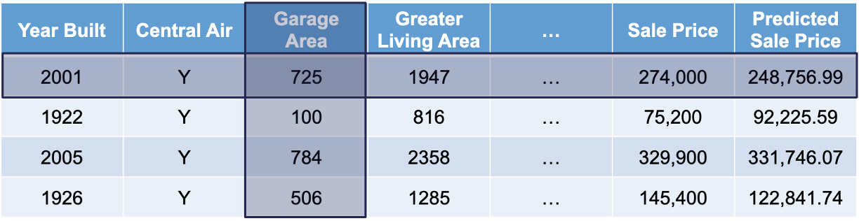{fig-align="center" width="11.65in"}Next, we will replicate this single observation over and over into a new dataset while holding all the other variables constant and not allowing their values to change. We will then fill in values for the variable of interest across the entire range of the variable: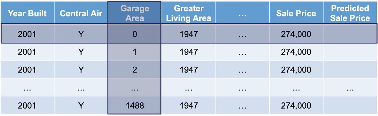{fig-align="center" width="11.65in"}Lastly, we will use the model to predict the target variable in each of these simulated observations: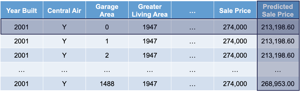{fig-align="center" width="11.65in"}This will give us an idea of how that single observation is impacted by that variable we are interested in. We will then repeat this calculation for each of the observations in our dataset (or a large sample of them).Let's see this in each of our softwares!::: {.panel-tabset .nav-pills}## RWe will continue to use the same random forest model from above. We still use the `Predictor$new` functionality of the `iml` package to build out the ICE for the random forest. We use the random forest model object as an input as well as the training dataset without the target variable, here column 1, in the `data` option. The `y =` option is where we specify the target variable, *Sale_Price*. The `type = 'response'` option tells R we want the predictions to be in the same scale as the continuous target variable.Lastly, we use the `FeatureEffects$new` function on this prediction object. We specify the method we want to use for our interpreter which is `method = 'ice'`. The `plot` element just plots the results. To specify a specific variable we can input that variable name into the plot function. Otherwise, it will produce ICE plots for all of the variables.```{r}#| warning: false#| error: false#| message: falselibrary(patchwork)set.seed(12345)forest_pred <- Predictor$new(rf.ames, data = training[,-1], y = training$Sale_Price, type ="response")ice_plot <- FeatureEffects$new(forest_pred, method ="ice")ice_plot$plot(c("Garage_Area"))ice_plot$plot()```Let's take a look at the results above. These plots have the possibility of overwhelming people the first time they see them. In reality, these plots don't serve too much value when you plot all of the lines on the same plot. As we can see with the *Garage_Area* plot, there are different patterns going on for different observations. ICE is a local method which is best used to just explore the plot of a single observation, or just examine the predictions of a single observation.## PythonWe will continue to use the same random forest model from above. To get our ICE calculation we will use the `skexplain` package from scikit-learn. We will use the `ExplainToolkit` function where we input our model (along with a name, `('Random Forest, rf_ames')`) as well as our predictor variables and target variable in the usual `X =` and `y=` options from scikit-learn.Next, we use the `ale` function on the above `ExplainToolkit` object. We want to see the calculation for a specific variable, *Garage_Area*. Next, we also use the `ice` function on the `ExplainToolkit` object with the same feature of interest. Lastly, we use the `plot_ale` function on the original `ExplainToolkit` object with the `ale` and `ice` objects serving as inputs to the `ale` and `ice_curves` options respectively. Again, we have to specify the model name, here in the `estimator_names` option. After a couple of label and figure options for viewing, we have our ICE plot.```{python}#| warning: false#| error: false#| message: falseexplainer = skexplain.ExplainToolkit(('Random Forest', rf_ames), X = X_train, y = y_train)ale = explainer.ale(features ='Garage_Area', n_bootstrap =2, n_bins=20)ice = explainer.ice(features ='Garage_Area', random_seed =12345)fig, axes = explainer.plot_ale( ale = ale, estimator_names ='Random Forest', ice_curves = ice, xlabels = ['Garage Area'], figsize=(5,4) )```Let's take a look at the results above. These plots have the possibility of overwhelming people the first time they see them. In reality, these plots don't serve too much value when you plot all of the lines on the same plot. As we can see with the *Garage_Area* plot, there are different patterns going on for different observations. There is also a histogram of the *Garage_Area* variable hidden in the background as well. ICE is a local method which is best used to just explore the plot of a single observation, or just examine the predictions of a single observation.:::One of the biggest disadvantages of ICE is the impact of multicollinearity. If the variable of interest is correlated with other predictor variables, some of the simulated data may be invalid. Let's take a look at *Garage_Area* across values of first floor square footage: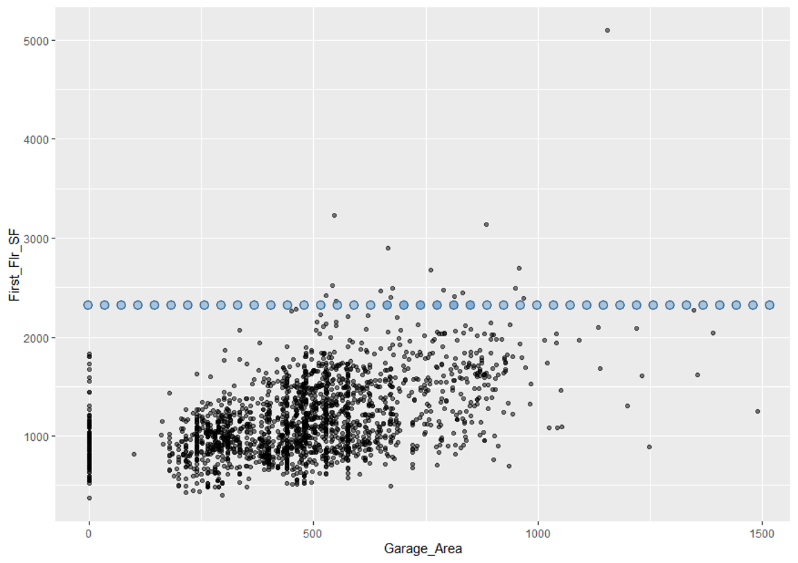{fig-align="center" width="5.68in"}Since we are fixing first floor square footage for a single observation and then simulating all of the possible values of *Garage_Area*, we could get some nonsensical values. As we can see by the horizontal dots above, a home with 2400 square feet on the first floor would reasonably have values of *Garage_Area* in between 500 and 1300 square feet. However, we are simulating these homes all the way down to no garage and up to values of 1500 square feet. Therefore, we must be careful when interpreting ICE predictions for a single observation as some of the predictions are extrapolating outside of the reasonable range of values.# Partial Dependence#### General Idea::: {.callout-tip appearance="simple"}"Let me show you what the model predicts on average when each observation has the value *k* for that feature, regardless if that value makes sense.":::A **partial dependence plot (PDP)** is a global interpreter that attempts to show the **marginal** effect of predictor variables on the target variable. Marginal effects are averaged effects over all possible values of a single variable. Essentially, the PDP is the average of the ICE plots discussed in the section above.Let's look at this concept visually. First, choose a variable of interest. We will look at *Garage_Area*. Next, we will replicate the entire dataset while holding all variables constant except for the variable of interest:{fig-align="center" width="11.65in"}Next, we will fill the variable of interest column in each dataset with one of the possible values (determined by the range of the data) of the predictor variable of interest: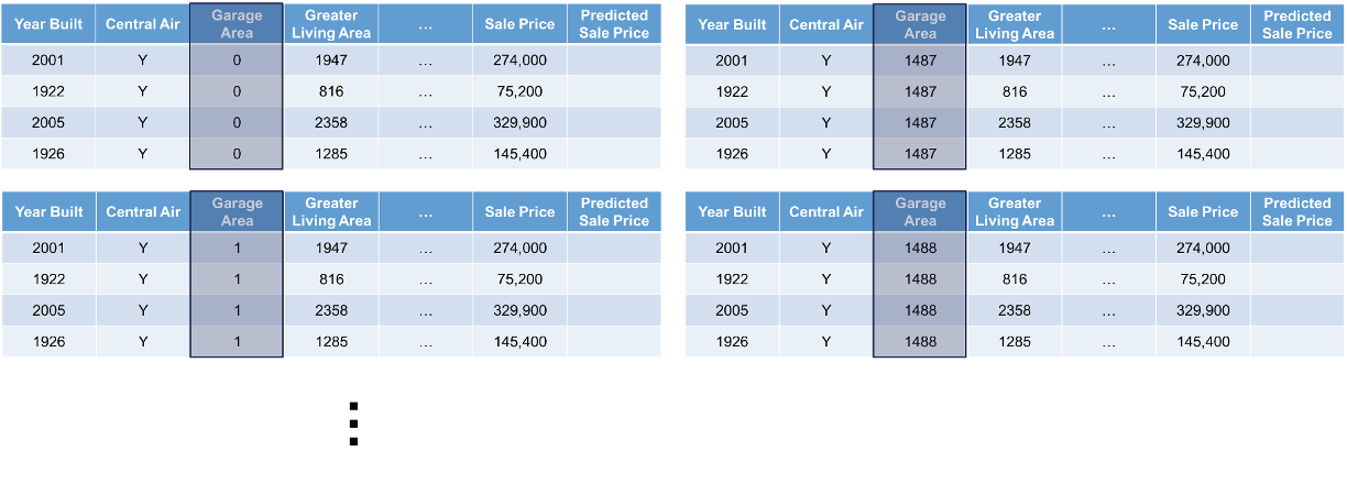{fig-align="center" width="11.65in"}We will use our model to generate predictions across all of the rows of each of the datasets. The predictions from each dataset will be averaged together and they will correspond to a particular value of the predictor variable of interest. That means we will have a dataset and prediction for each of the values in the range of *Garage_Area* which is 0 to 1488: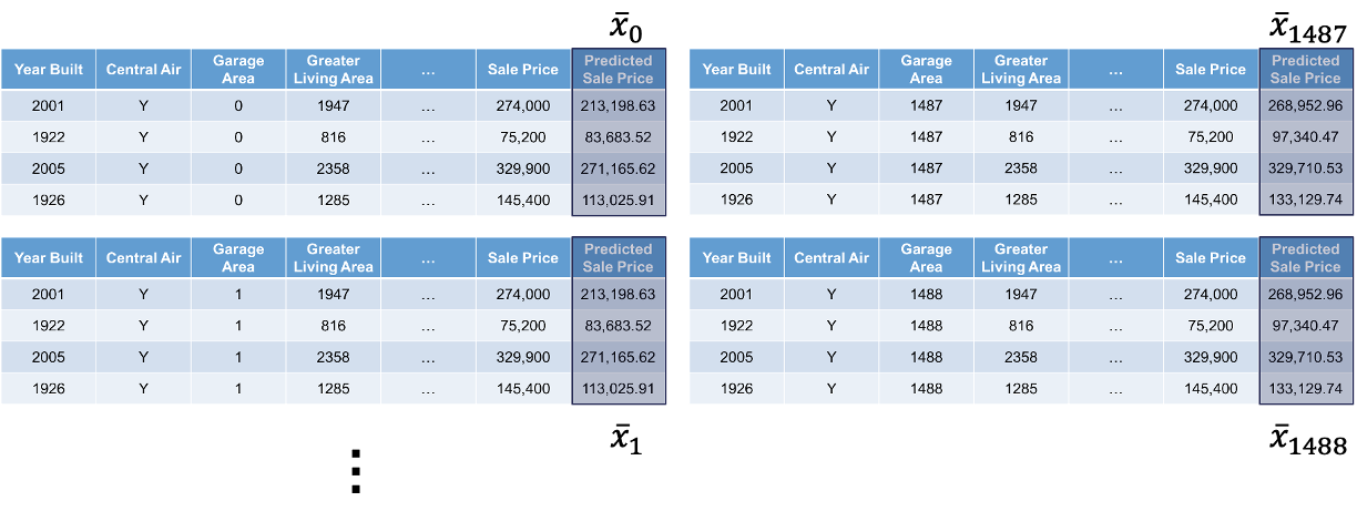{fig-align="center" width="11.65in"}This will give us an idea of how that are target variable is impacted on average by that variable we are interested in. The visual of this will hopefully show the potentially complex relationship between that predictor variable and the target variable.Let's see this in each of our softwares!::: {.panel-tabset .nav-pills}## RWe will continue to use the same random forest model from above. We still use the `Predictor$new` functionality of the `iml` package to build out the PDP for the random forest. We will not repeat all the code for the `Predictor$new` function as it is listed above.We use the `FeatureEffects$new` function on this prediction object from the `Predictor$new` function. We specify the method we want to use for our interpreter which is `method = 'pdp'`. The `plot` element just plots the results. To specify a specific variable we can input that variable name into the plot function. Otherwise, it will produce PDP plots for all of the variables.```{r}#| warning: false#| error: false#| message: falsepd_plot <- FeatureEffects$new(forest_pred, method ="pdp")pd_plot$plot(c("Garage_Area"))pd_plot$plot()```This nonlinear and complex relationship between *Garage_Area* and *Sale_Price* is similar to the plot we saw earlier with the GAMs, random forests, and XGBoost model sections. This shouldn’t be too surprising. All of these algorithms are trying to relate these two variables together, just in different ways.If we wanted to see the PDP plotted on top of the ICE plots to get a better sense of what we are averaging to get the PDP line we can just switch the `method = 'pdp'` option to `method = 'pdp+ice'`.```{r}#| warning: false#| error: false#| message: falsepdice_plot <- FeatureEffects$new(forest_pred, method ="pdp+ice")pdice_plot$plot(c("Garage_Area"))pdice_plot$plot()```## PythonWe will continue to use the same random forest model from above. To get our PDP calculation we will use the `skexplain` package from scikit-learn and the `ExplainToolkit` function. We will not repeat all the code for the `ExplainToolkit` function as it is listed above.To get the PDP we use the `pdp` function on the above `ExplainToolkit` object. We want to see the calculation for a specific variable, *Garage_Area*. However, we are not limited to just viewing one at a time so we put two additional variables to see their PDP values as well. Lastly, we use the `plot_pdp` function on the original `ExplainToolkit` object with the `pd` object serving as input to the `pd` option.```{python}#| warning: false#| error: false#| message: falseimp_vars = ['Garage_Area', 'Year_Built', 'Gr_Liv_Area']pd = explainer.pd(features = imp_vars)fig, axes = explainer.plot_pd(pd = pd, figsize=(8,4))```This nonlinear and complex relationship between *Garage_Area* and *Sale_Price* is similar to the plot we saw earlier with the GAMs, random forests, and XGBoost model sections. This shouldn’t be too surprising. All of these algorithms are trying to relate these two variables together, just in different ways.:::One thing you should always be careful of when plotting our PDPs is the scale of the data. Most plotting functions across softwares will adjust the scale of the plot for you. This is not always helpful. Take a look at the plot below with the variable describing the month in which is the house is sold.```{r}#| warning: false#| error: false#| message: falsepd_plot$plot(c("Mo_Sold"))```This looks like there is a big change across different months of the year. However, if we focus on the y-axis, we see that these changes all occur within a couple of thousand dollars.# Accumulated Local Effects (ALE)#### General Idea::: {.callout-tip appearance="simple"}"Let me show how the model predictions change when I change the variables of interest to values within a small interval around their current values.":::Partial dependence plots are an average of ICE plots which we previously discussed have problems with multicollinearity. If the variable of interest is correlated with other predictor variables, some of the simulated data may be invalid. Let's take a look at *Garage_Area* across values of first floor square footage:{fig-align="center" width="5.68in"}Since we are fixing first floor square footage for a single observation and then simulating all of the possible values of *Garage_Area*, we could get some nonsensical values. As we can see by the horizontal dots above, a home with 2400 square feet on the first floor would reasonably have values of *Garage_Area* in between 500 and 1300 square feet. However, we are simulating these homes all the way down to no garage and up to values of 1500 square feet.Instead of looking at all values like ICE, and therefore PDP, the **accumulated local effects (ALE)** global interpreter uses only reasonably contrived data to get a clearer picture of the relationship between a variable of interest and the target variable. By default, ALE uses quantiles of your data to define this reasonable range of values. For observations in each interval, we determine how much their prediction would change if we replace the feature of interest with the upper and lower bounds of the interval, while keeping all other variables constant. Let's look at his visually: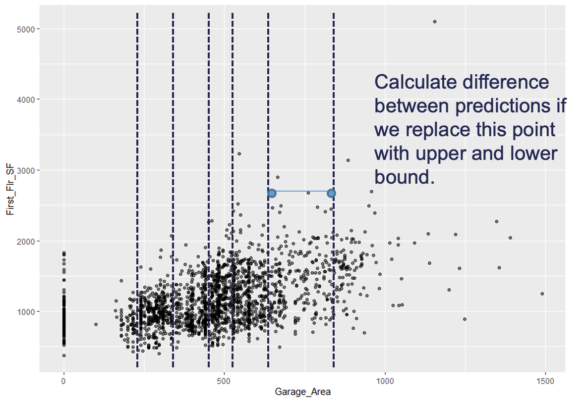{fig-align="center" width="5.68in" height="4in"}With the ALE we will do this calculation for all of the observations in the interval. This allows us to understand how the predictions are changing within a reasonable window around the data values for the predictor variable.Let's see how to do this in each of our softwares!::: {.panel-tabset .nav-pills}## RWe will continue to use the same random forest model from above. We still use the `Predictor$new` functionality of the `iml` package to build out the ALE for the random forest. We will not repeat all the code for the `Predictor$new` function as it is listed above.We use the `FeatureEffects$new` function on this prediction object from the `Predictor$new` function. We specify the method we want to use for our interpreter which is `method = 'ale'`. The `plot` element just plots the results. To specify a specific variable we can input that variable name into the plot function. Otherwise, it will produce ALE plots for all of the variables.```{r}#| warning: false#| error: false#| message: falseale_plot <- FeatureEffects$new(forest_pred, method ="ale")ale_plot$plot(c("Garage_Area"))ale_plot$plot()```The ALE curve that is provided is a centered calculation. This means that the ALE describes the main effect of the predictor variable **compared to the data's average prediction**. For example, in the plot above for *Garage_Area*, the value of 700 square feet for *Garage_Area* corresponds to a value of \$10,000 in ALE. This means that when Garage_Area is 700 square feet, the prediction for our sale price is \$10,000 higher than the average prediction in our model.Another interesting point to observe on an ALE plot is the spot where the values go from negative to positive. Again, using the *Garage_Area* plot above, we see that around 500 square feet of *Garage_Area* the effect on the prediction of sale price of the home changes from negative to positive. Therefore, homes with values smaller than 500 square feet lead to a below average prediction as compared to homes above 500 square feet have an above average prediction.## PythonWe will continue to use the same random forest model from above. To get our ALE calculation we will use the `skexplain` package from scikit-learn and the `ExplainToolkit` function. We will not repeat all the code for the `ExplainToolkit` function as it is listed above.To get the ALE we use the `ale` function on the above `ExplainToolkit` object. We want to see the calculation for a specific variable, *Garage_Area*. However, we are not limited to just viewing one at a time so we put two additional variables to see their ALE values as well. Lastly, we use the `plot_ale` function on the original `ExplainToolkit` object with the `ale` object serving as input to the `ale` option.```{python}#| warning: false#| error: false#| message: falseimp_vars = ['Garage_Area', 'Year_Built', 'Gr_Liv_Area']ale = explainer.ale(features = imp_vars)fig, axes = explainer.plot_ale(ale = ale, figsize=(8,4))```The ALE curve that is provided is a centered calculation. This means that the ALE describes the main effect of the predictor variable **compared to the data's average prediction**. For example, in the plot above for *Garage_Area*, the value of 700 square feet for *Garage_Area* corresponds to a value of \$10,000 in ALE. This means that when Garage_Area is 700 square feet, the prediction for our sale price is \$10,000 higher than the average prediction in our model.Another interesting point to observe on an ALE plot is the spot where the values go from negative to positive. Again, using the *Garage_Area* plot above, we see that around 500 square feet of *Garage_Area* the effect on the prediction of sale price of the home changes from negative to positive. Therefore, homes with values smaller than 500 square feet lead to a below average prediction as compared to homes above 500 square feet have an above average prediction.:::# Local Interpretable Model-Agnostic Explanations (LIME)#### General Idea::: {.callout-tip appearance="simple"}"Let me show you a linear model that could explain the exact orientation of the predictive model at a specific point.":::The best way to understand the local interpreter LIME is through a visual. Imagine that you had a nonlinear relationship between a target and a predictor variable. Now imagine you zoom in really close to a specific point of interest as in the figure below: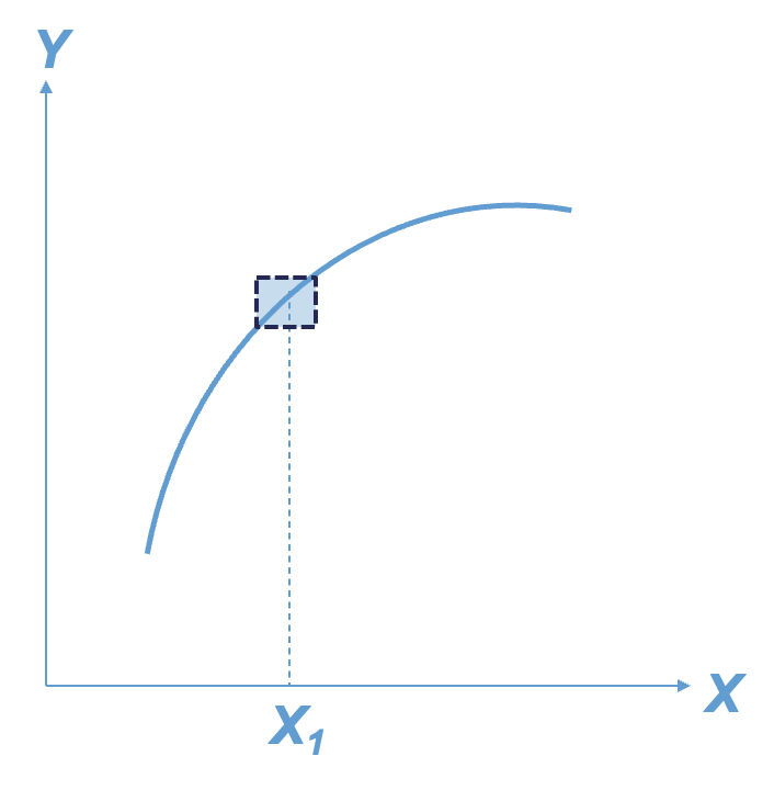{fig-align="center" width="3.93in"}That zoomed in area around the point of interest looks like an approximately straight line. We know that we can model (and interpret) straight lines with linear regression. This will help us understand the effects or impact of that variable of interest around our point of interest. Of course, we can expand this linear regression to include all of the variables and not just one.Here are the basic steps of what LIME is doing:1. Randomly generate values (usually, normally distributed) for each variable in the model.2. Weight more heavily the fake observations that are **near the real observation of interest**.3. Build a **weighted** linear regression model based on fake observations and the observation (row in the dataset) of interest.4. "Interpret" the coefficients of variables and their "impact" from the linear regression model.LIME is not actually limited to linear regression and we could use any interpretable model (decision tree for example). One of the biggest choices we have in LIME is the number of variables we use in the local linear regression model. Typically, we don't use all of the variables in a local model like LIME as we are trying to focus on the main driving factors. However, the definition of "near the points of interest" is a very big and **unsolved** problem in the world of LIME.Let's see how to do this in each of our softwares!::: {.panel-tabset .nav-pills}## RWe will continue to use the same random forest model from above. We still use the `Predictor$new` functionality of the `iml` package to build out the LIME for the random forest. We will not repeat all the code for the `Predictor$new` function as it is listed above.For LIME we will use the `LocalModel$new` function. We will still use the same `Predictor$new` object from above in this function. The only other input is the specific observation that we want to "interpret," which is observation number 1328 in the example below. The `k = 5` option tells the LIME process to use only use 5 variables for the local model. We can look at both a plot of the results (using the `plot` function) or just the LIME results directly by looking at the `results` element of the `LocalModel$new` object.```{r}#| warning: false#| error: false#| message: falsepoint <-1328lime.explain <- LocalModel$new(forest_pred, x.interest = training[point,-1], k =5)plot(lime.explain) +theme_bw()lime.explain$results```Let's first examine the plot. The bars in the plot represent the "effect" of the variables. This effect is the slope of the linear regression for that variable multiplied by the values of the variable itself, essentially $\beta_i x_i$. The tabular results can help us see this a little more. For example, the *Year_Built* variable has a slope coefficient for the local regression of 647.22. This house specifically was built in 1994. That means the "effect" of that variable is 1,290,551.21. The biggest takeaways from the plot above is the variables that have the most "effect." Notice that the *Fireplaces* variable has the biggest slope for the local regression, but since it take a value of 2, the "effect" for this observation is still smaller than other variables.Let's take a look at how this might change for another observation. Instead of observation 1328, let's explore observation 1000 with the same code.```{r}#| warning: false#| error: false#| message: falsepoint <-1000lime.explain <- LocalModel$new(forest_pred, x.interest = training[point,-1], k =5)plot(lime.explain)```From the above output we can see that the variable *Year_Built* still has the greatest effect on our prediction, but the order and magnitude of the variables is different because this is a different, local linear regression.## PythonFor LIME we are going to use a different package in Python, namely the `lime` package. From the `lime` package we will import the `lime_tabular` package. From this set of packages we will use the `LimeTabularExplainer` function which has an array of inputs we need to fill in. The first input is the values from your training dataset. Since our dataset is a data frame, we will use the `.values` function to extract just the values. We then need to give the function the names of the training dataset variables in the `feature_names` option using the `columns` function on our training data frame. The `class_names` option is where we specify the name of the target variable. Next, we need to give the function the names of the categorical variables with the `categorical_features` option. Lastly, we need to specify the `mode = 'regression'` option so the model knows the input is a regression model and not a classification model.Now that we have our `LimeTabularExplainer` object defined, we can use the `explain_instance` function on this object. The inputs to the `explain_instance` function are the specific observation you are interested in, here observation 1328, the predictions from our random forest model (using the `predict` function), and the number of variables we want in the local regression. The results from the LIME model can be seen in either a list using the `as_list()` function or in a plot using the `as_pyplot_figure()` option.```{python}#| warning: false#| error: false#| message: falseimport limefrom lime import lime_tabularexplainer = lime.lime_tabular.LimeTabularExplainer( X_train.values, feature_names = X_train.columns, class_names = ['Sale_Price'], categorical_features = [X_train.columns.get_loc(col) for col in ['Street_Grvl', 'Street_Pave', 'Central_Air_N', 'Central_Air_Y']], verbose =True, mode ='regression')exp = explainer.explain_instance(X_train.values[1327], rf_ames.predict, num_features =5)exp.as_list()exp.as_pyplot_figure()```Let's first examine the plot. The bars in the plot represent the "effect" of the variables. This effect is the slope of the linear regression for that variable multiplied by the values of the variable itself, essentially $\beta_i x_i$. Since all of these "effects" are from a linear regression, we can add them together to get the predicted value from the local linear regression. This truly allows us to see how the prediction is broken down by each variable. We can see this even more with the list output. We can see the intercept from the linear regression along with the "effects" of each of the variables. These added together sum up to the predicted value listed in the output as well.The biggest takeaways from the plot above is the variables that have the most "effect" locally on that observation. This could change for each observation. Instead of observation 1328, let's explore observation 1000 with the same code.```{python}#| warning: false#| error: false#| message: falseexp = explainer.explain_instance(X_train.values[999], rf_ames.predict, num_features =5)exp.as_list()exp.as_pyplot_figure()```From the above output we can see that the variable *Year_Built* still has the greatest effect on our prediction, but the order and magnitude of the variables is different because this is a different, local linear regression. We can even see with this observation that some of the variables had a negative impact on our predicted sale price. For example, the smaller first floor square footage actually decreased our sale price prediction locally by almost \$18,900.:::# Shapley Values#### General Idea::: {.callout-tip appearance="simple"}"Let me show you the value the $j^{th}$ feature contributed to the prediction of this particular observation compared to the average prediction of the whole dataset.":::As mentioned above, the general idea for the Shapley value local interpreter is to measure the "effect" of a specific variable on the difference in the prediction of a specific point compared to the overall prediction. This is best seen through an example. In Python, the predicted sale price of observation 1328 is \$672,791.28 from our random forest. The average, predicted sale price of homes from the random forest is \$180,628.03. Let's now look at the Shapley values for observation 1328: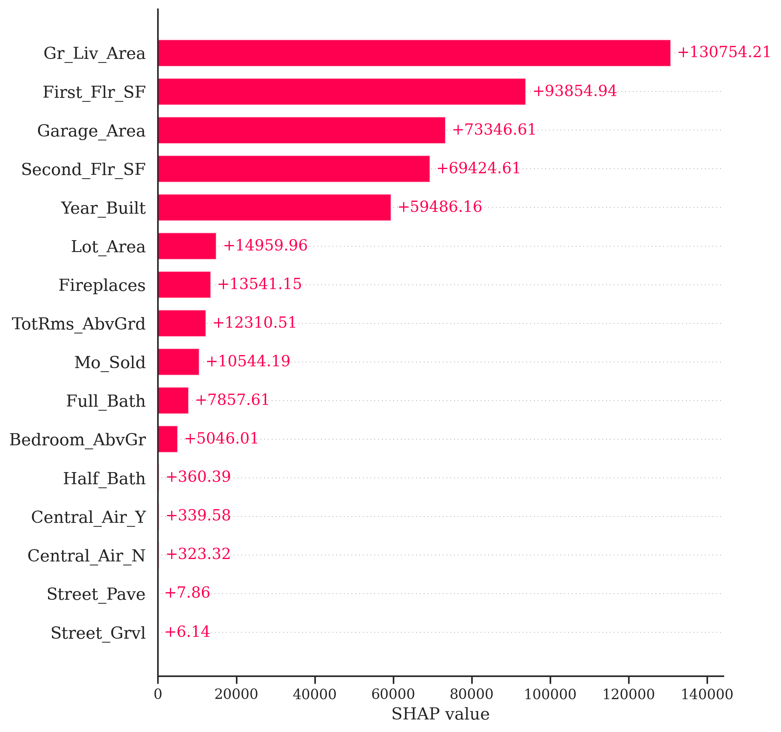{fig-align="center" width="5in"}If we were to take all of the pieces you see above and sum them together, $13,754.21 + 93,854.94 + \cdots + 6.14 = 492,163.25$. This is the exact difference between our predicted value of \$672,791.28 and the overall prediction of \$180,628.03. This means we can directly see how each variable impacts our specific prediction of observation 1328 in terms of the predicted sale price of the home.This sounds great, but how does it work in the background? It goes back to the mathematical idea of game theory. Shapley (1953) assigned a payout values for players depending on their contribution to the total payout across a coalition (think team). In other words, imagine you have a team of basketball players playing in a local tournament. You all win some money in the local tournament. How do you split the winnings? Evenly? Maybe. Or you could split the winnings based on contribution to the team. The star player gets the most, followed by the second best player, and so on all the way down the team. That is the idea of a Shapley value in game theory.The Shapley value in machine learning is the average marginal contribution of a variable / feature (teammate) across all possible coalitions of variables (possible combinations of teammates). For this we would need to compute the average change in the prediction that a set of variables experiences when the variable of interest is added to the coalition. This computation is done across all observations and across all possible combinations of variables. This calculation can be very time consuming to do with large numbers of variables. There has been a tremendous amount of research in machine learning on how to accomplish this calculation much quicker, such as sampling, subsets of variables, etc.The creators of Shapley values in machine learning tout four factors for Shapley values that, they argue, makes it one of the best local interpreters.1. Efficiency - variable contributions must sum to the difference of the prediction for the point of interest compared to the average prediction.2. Symmetry - contributions of two variables should be the same if they contribute equally to all possible combinations of variables.3. Dummy - a variable that does not change the predicted value, for any combination of variables, should have a Shapley value of 0.4. Additivity - for a forest of trees, the Shapley value of the forest for a given observation should be the average of the Shapley values for each tree at that given point.Let's see this in each of our softwares!::: {.panel-tabset .nav-pills}## RWe will continue to use the same random forest model from above. We still use the `Predictor$new` functionality of the `iml` package to build out the Shapley values for the random forest. We will not repeat all the code for the `Predictor$new` function as it is listed above.We will input the `Predictor$new` object into the `Shapley$new` function. The only other option we need to specify is the specific observation we are interested in. Here we will look at observation 1328 like we did with LIME. All we need to input is the training dataset predictor values at that specific point. Lastly, we just call the `plot()` function on that `Shapley$new` object to visualize the values.```{r}#| warning: false#| error: false#| message: falsepoint <-1328shap <- Shapley$new(forest_pred, x.interest = training[point,-1])shap$plot()```Similar to the Python example worked out above, this plot gives us the overall prediction of sale price across the whole dataset as well as the specific prediction of observation 1328 from our random forest. The bars in the plot represent the impact that a variable has in the difference between that average prediction and the specific prediction of the point. We can see that the *Gr_Liv_Area* variable has the greatest impact on the difference in prediction.Let's take a look at how this might change for another observation. Instead of observation 1328, let's explore observation 1000 with the same code.```{r}#| warning: false#| error: false#| message: falsepoint <-1000shap <- Shapley$new(forest_pred, x.interest = training[point,-1])shap$plot()```From the above plot we can see drastically different effects for this observation compared to observation 1328. Here, the *Year_Built* variable has the greatest **positive** impact on the difference in predicted sales price. However, this observation also has some values that are negatively impacting our prediction. For example, the small first floor square footage appears to have a strong **negative** impact on our prediction.## PythonFor Shapley values we will need to use a different package in Python, the `shap` package. We are also loading in `matplotlib.pyplot` for some of the plotting options on the Shapley values. From the `shap` library we need the `Explainer` function. The input to this function is the random forest model we have previously built. With this new `Explainer` object we input the predictor variables from the training dataset to get the Shapley values.```{python}#| warning: false#| error: false#| message: falseimport shapimport matplotlib.pyplot as pltexplainer = shap.Explainer(rf_ames)shap_values = explainer(X_train)```Now that we have the Shapley values we can visualize them in a variety of ways. First, we have a bar plot of the impact of the individual variables on the difference in prediction. For this we just use the `shap.plots.bar` function on the Shapley values object. Specifically, we are looking at observation 1328. We also use the `max_display` option to determine how many variables are plotted. By default, this takes a value of 10, but we want to see all of the variables.```{python}#| warning: false#| error: false#| message: false#| eval: falseshap.plots.bar(shap_values[1327], max_display =16)```{fig-align="center" width="5in"}Exactly as the original example worked out above, the bars in the plot represent the impact that a variable has in the difference between that average prediction across all houses form the random forest and the specific prediction of observation 1328. We can see that the *Gr_Liv_Area* variable has the greatest impact on the difference in prediction.Let's take a look at how this might change for another observation. Instead of observation 1328, let's explore observation 1000 with the same code.```{python}#| warning: false#| error: false#| message: false#| eval: falseshap.plots.bar(shap_values[999], max_display =16)```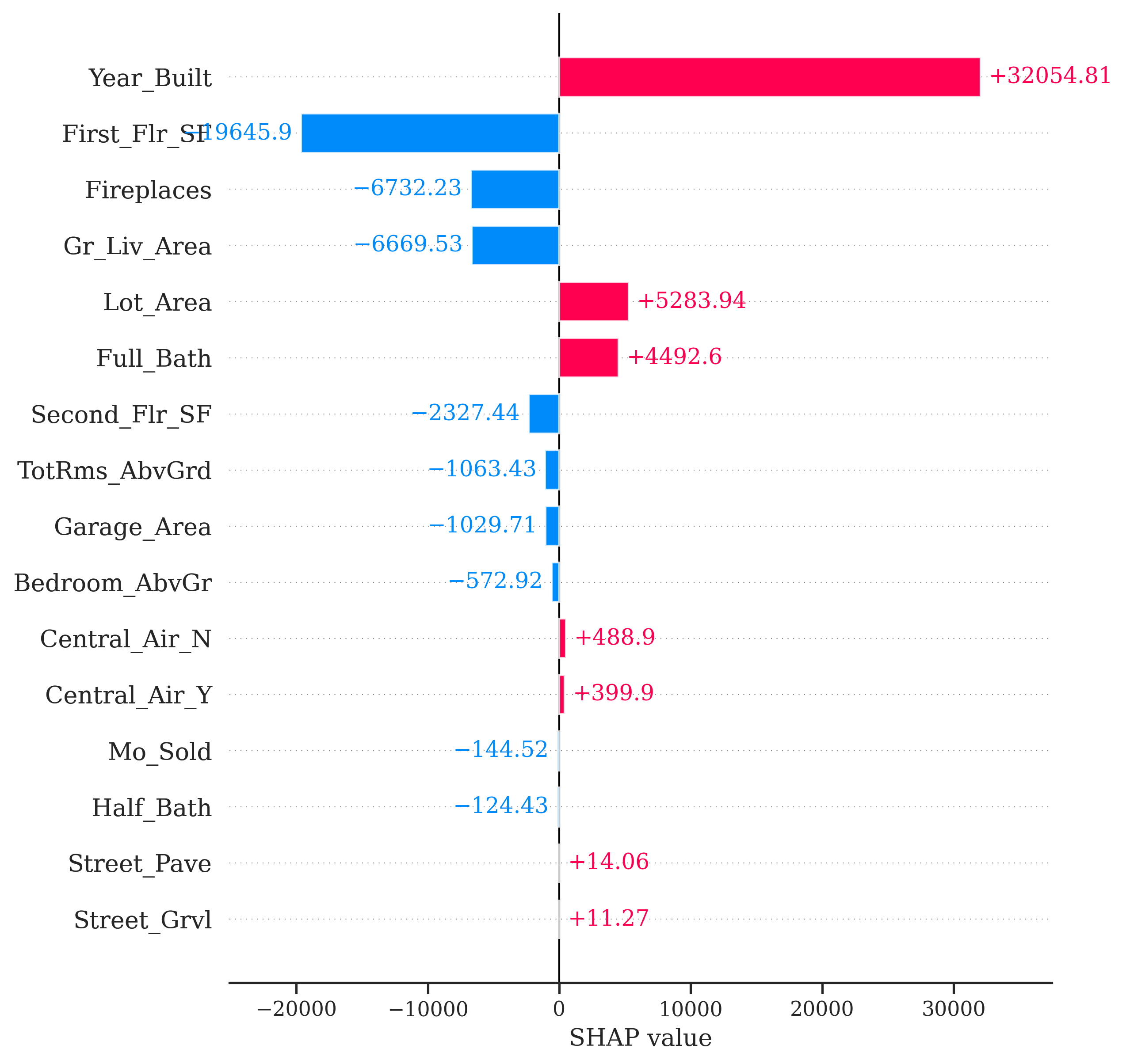{fig-align="center" width="5in"}From the above plot we can see drastically different effects for this observation compared to observation 1328. Here, the *Year_Built* variable has the greatest **positive** impact on the difference in predicted sales price. However, this observation also has some values that are negatively impacting our prediction. For example, the small first floor square footage appears to have a strong **negative** impact on our prediction.:::## CautionsThere are some things to be cautious about with Shapley values. Some people try to look at the "overall impact" of a variable across all of the observations. One should be very careful with this approach as Shapley values were designed for local interpretations, not necessarily global ones.For example, in Python we can use the `shap.plots.bar` function on all of the Shapley values instead of a specific one. This plot will show us the average of the absolute value of all of the Shapley values for a variable.```{python}#| warning: false#| error: false#| message: false#| eval: falseshap.plots.bar(shap_values, max_display =16)```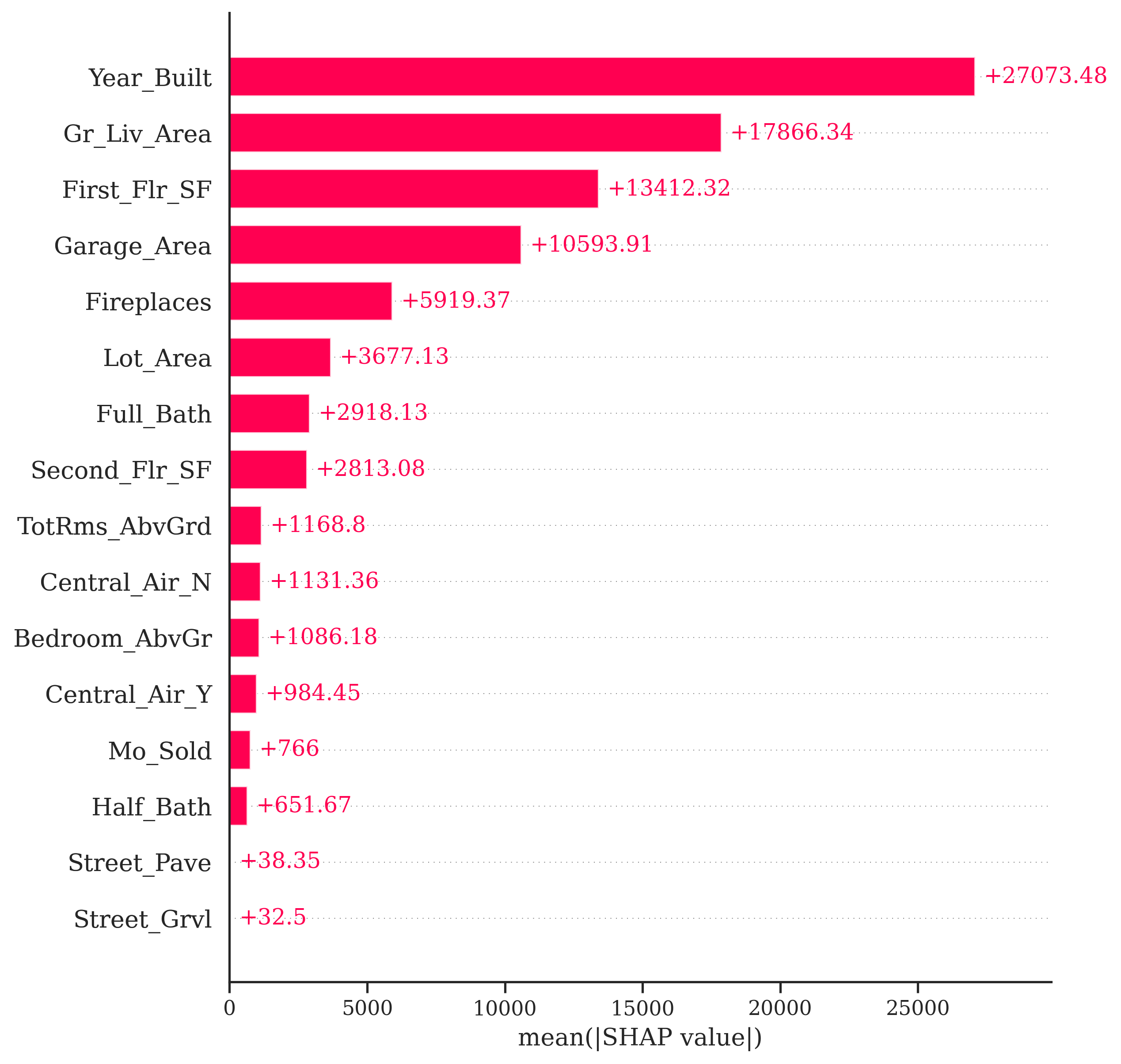{fig-align="center" width="5in"}One potentially valuable piece of information from the plot above is to see that the variable *Gr_Liv_Area* has the largest average magnitude of impact compared to the other variables. However, this number doesn't necessarily capture the variability of the impact. We should not assume that all of the impacts are positive (remember, this is an absolute value) or that all of the observations have this specific impact. We saw in our two examples above that some variables have a positive and negative effect on different observations and there are definitely different magnitudes of impact of the same variable on different observations.Another common plot you will see with Shapley values is the bee swarm plot from the `shap.plots.beeswarm` function applied to all Shapley values. This tries to show the variability of the impact of each variable across many different observations. Really, the only value form this plot is that notion of variation, but rarely have I noticed clients understanding or needing this plot. One should be hesitant to share this plot with any non-technical audience.```{python}#| warning: false#| error: false#| message: false#| eval: falseshap.plots.beeswarm(shap_values, max_display =16)```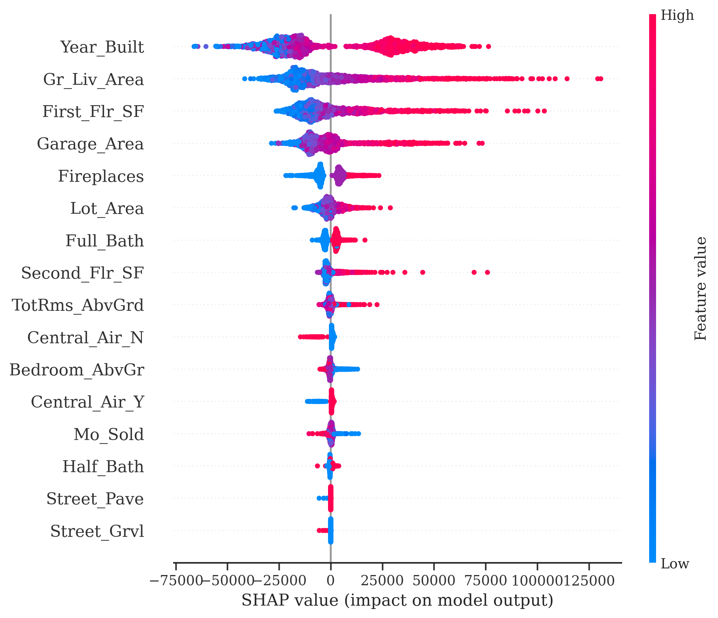{fig-align="center" width="5in"}